Donald R. van Deventer[1]
First Version: October 19, 2021
This Version: October 21, 2021
ABSTRACT
Please note: Kamakura Corporation term structure models are updated monthly. For the most recent set of coefficients, contact info@kamakuraco.com
This paper analyzes the number and the nature of factors driving the movements in government yield curves from 13 countries from January 2, 1962 through September 30, 2021. The countries included are Australia, Canada, France, Germany, Italy, Japan, Russia, Singapore, Spain, Sweden, Thailand, the United Kingdom, and the United States. There are four primary reasons for constructing a composite “World” term structure model. First, as shown in the paper, the vast majority of the 13 countries do not have the same breadth (years to maturity span) and depth (length of the time series) as a consolidated model. Second, the spread of negative interest rates in many government markets is crucial data for those countries with no negative rate experience. Third, even if all countries had an equal amount of data, Stein’s paradox and modern empirical Bayes approaches prove that such a consolidated model will produce more accurate results than the stand-alone single country models. Finally, the consolidated data set is six times larger than the U.S. Treasury history, with more than 90,000 observations. This large data set results in simulated yield curves that are more realistic in their shapes and in their evolution than a smaller data set can produce.
PDF Version:
Kamakura-AnUpdatedHJMModelfor13Countriesv1-20211021
A 12-Factor Heath, Jarrow, and Morton Stochastic Volatility Model
For 13-Country `World’ Government Bonds,
Using Daily Data from January 1, 1962 through September 30, 2021
This paper analyzes the number and the nature of factors driving the movements in government yield curves from 13 countries from January 2, 1962 through September 30, 2021. The countries included are Australia, Canada, France, Germany, Italy, Japan, Russia, Singapore, Spain, Sweden, Thailand, the United Kingdom, and the United States. This list of countries is composed of 11 members of the G20 group plus Sweden and Thailand.
There are four primary reasons for constructing a composite “World” term structure model. First, as shown in the paper, the vast majority of the 13 countries do not have the same breadth (years to maturity span) and depth (length of the time series) as a consolidated model. Second, the spread of negative interest rates in many government markets is crucial data for those countries with no negative rate experience. Third, even if all countries had an equal amount of data, Stein’s paradox and modern empirical Bayes approaches prove that such a consolidated model will produce more accurate results than a stand-alone single country model. Finally, the consolidated data set is six times larger than the U.S. Treasury history, with more than 90,000 observations. This large data set results in simulated yield curves that are more realistic in their shapes and in their evolution than a smaller data set can produce.
Section I discusses the origin and characteristics of the daily data base of government yields from the 13-country data set. We discuss yield curve smoothness and volatility fitting as measures for judging the quality of government-generated yield curve time series and present an example of the technique in this paper. We conclude that the 13-country data set is an exceptionally rich collection of yield curves with negative rates. Significant cleansing of the database was necessary, particularly for data from Japan, Sweden, Spain, and Thailand.
Section II outlines the process for determining whether the interest rate volatility functions for the factors driving the 13-country yield curves are constants (an “affine” model) or stochastic, typically expressed as a function of the level of interest rates. Section III describes the process of fitting five different Heath, Jarrow, and Morton models to the 13-country yield data: models with 1, 2, 3, 6 and 12 factors. We conclude Section III with extensive Bayesian model validation procedures based on a 30-year forward-looking simulation of 500,000 scenarios, using both World and single-country parameters, for the U.S. Treasury curve on October 15, 2021. Section IV concludes the paper. Appendix A illustrates a sample model validation process for widely used one-factor term structure models using World data. Appendix B includes an analysis of empirical drift and stress tests of rate volatility. Appendix C compares the span of interest rates by level and months to maturity for the World data set versus the 13 countries which contributed data to the consolidated yield data base.
I. 13-Country Yield Data: Special Characteristics
A multi-factor term structure model is the foundation for best practice asset and liability management, market risk, economic capital, interest rate risk in the banking book, stress-testing, and the internal capital adequacy assessment process. The objective in this paper is to illustrate the derivation of a multi-factor Heath Jarrow and Morton model of the yield curve data from 13 countries. As a by-product, the analysis has the potential to detect common data problems associated with yield curve histories and employs a standard methodology for quantification and resolution of those problems. Previous implementations of multi-factor Heath, Jarrow, and Morton models have covered the following bond market sectors:
- Australia Commonwealth Government Securities
- Canada Government of Canada Securities
- France French Government Securities
- Germany German Bunds
- Italy Italian Government Securities
- Japan Japanese Government Bonds
- Russia Russian Government Securities
- Singapore Singapore Government Securities
- Spain Spanish Government Bonds
- Sweden Swedish Government Securities
- Thailand Thai Government Securities
- United Kingdom United Kingdom Government Bonds
- United States U.S. Treasury Securities
The first step in data model validation for the 13-country data set is to examine the historical availability of bond yields over time. This availability is summarized in Table I. Because there are more than 200 different data regimes in the data set, the table is broken into 7 sub tables:
Table I


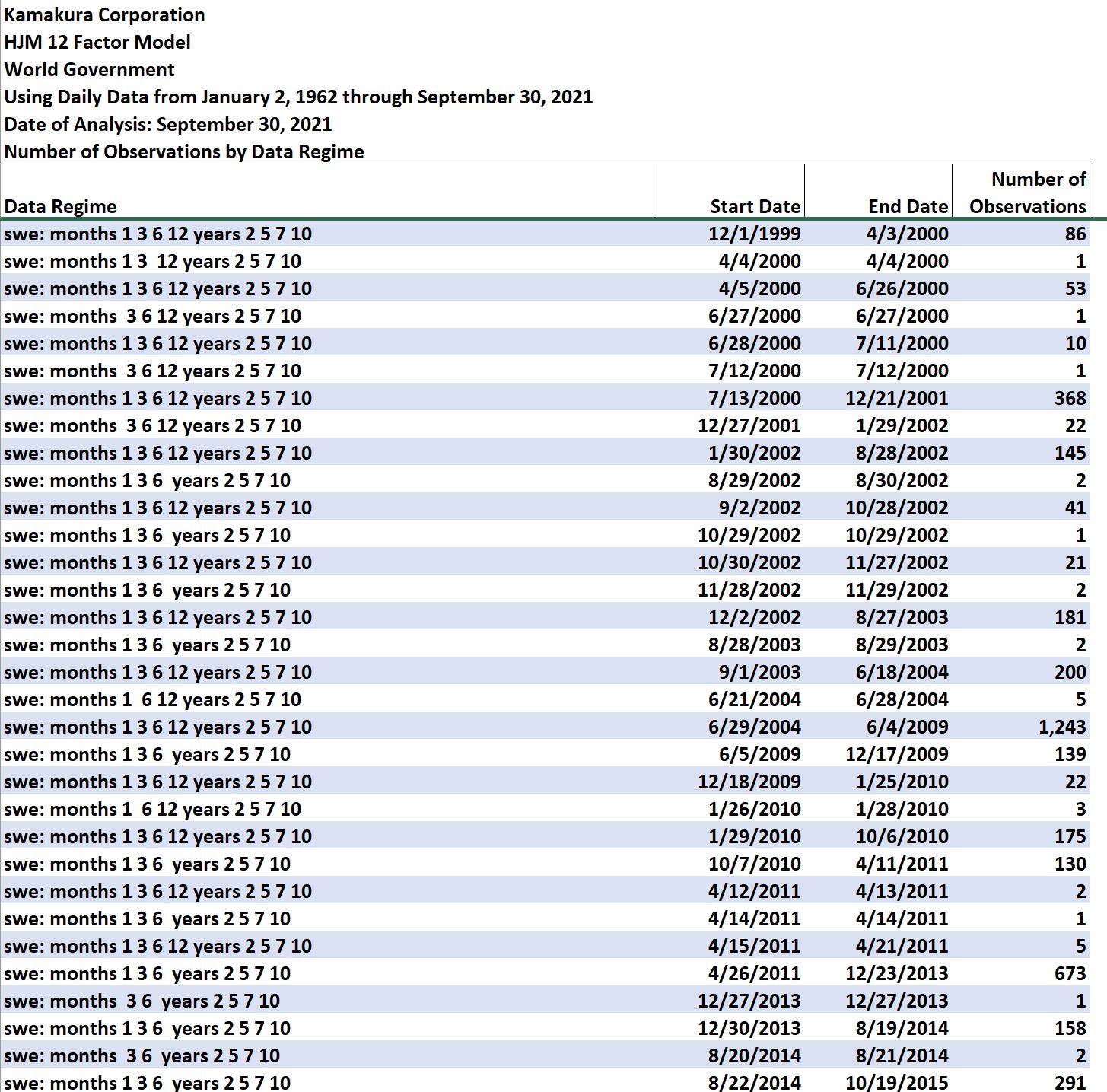

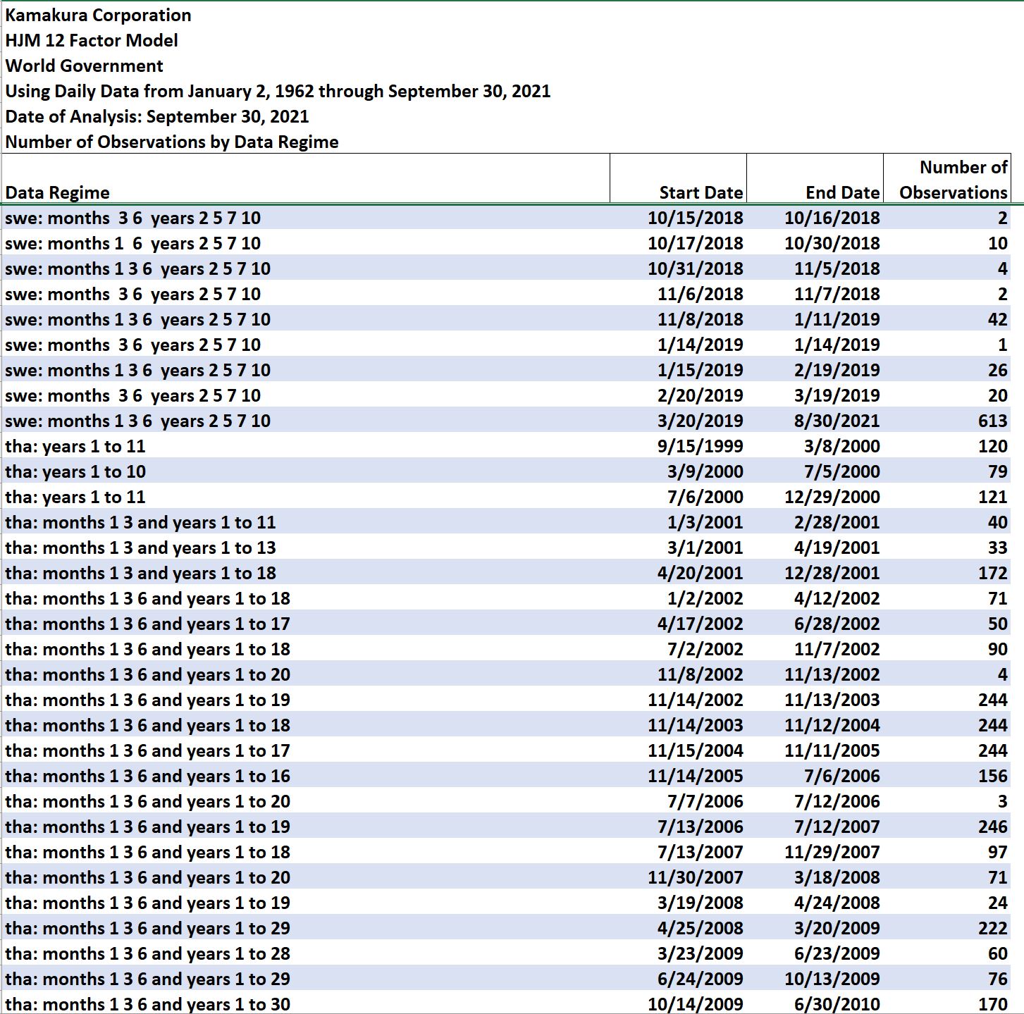
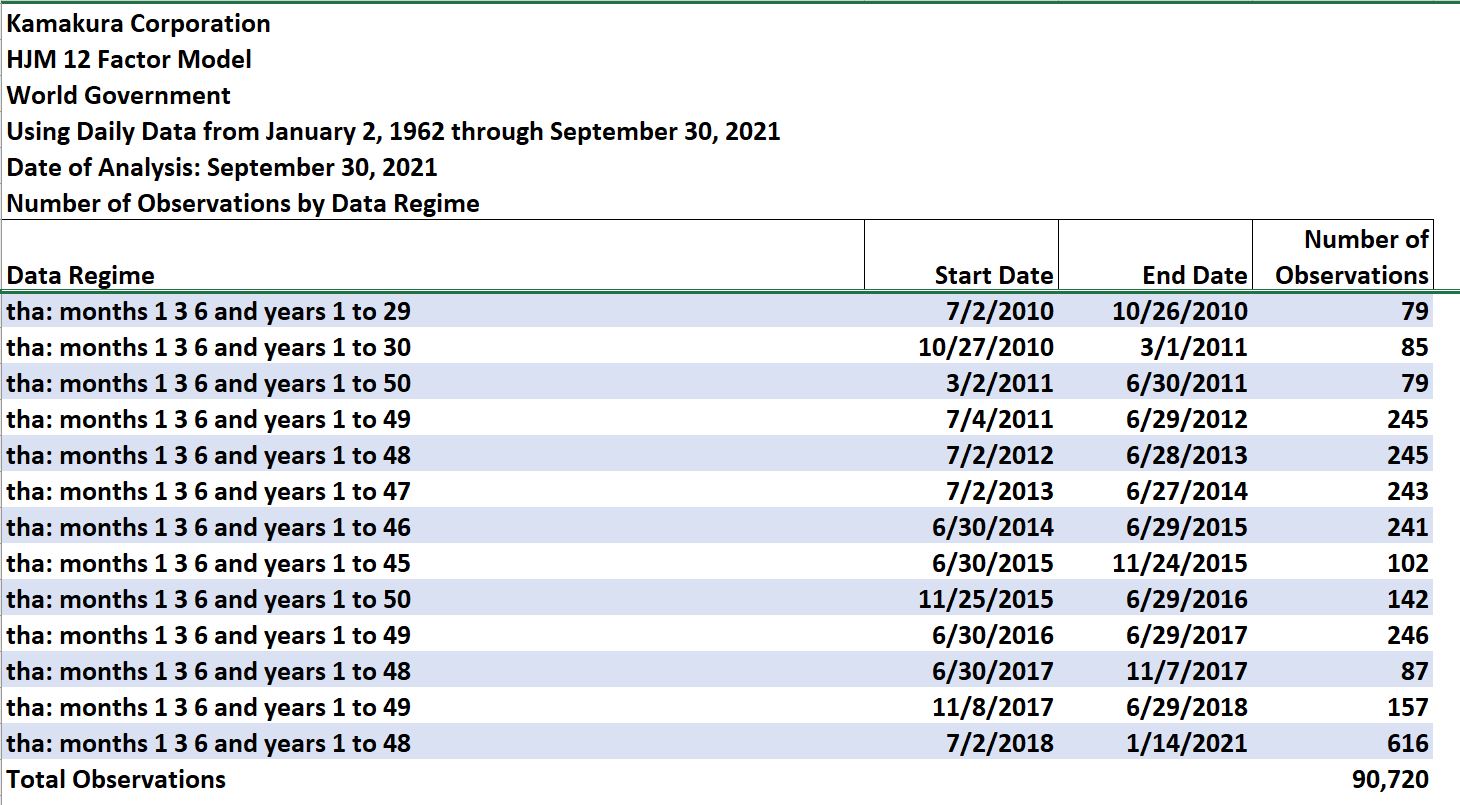
Sweden and Thailand account for the very large number of data regimes in the 13-country data set. We discuss the implications of this for modeling strategy below.
Because our Heath, Jarrow and Morton analysis makes use of a yield curve with 91-day (quarterly) forward rate segments, the next step in data model validation is to fit 91-day forward rates to the raw coupon-bearing bond yields. The smoothness of the resulting forward rates will be a function of both the quality of the raw data from a smoothness point of view and the smoothness implied by the secondary smoothing process. To ensure the maximum smoothness from the secondary smoothing process, we use the maximum smoothness forward rate methodology of Adams and van Deventer [1994], as corrected in van Deventer and Imai [1996]. Adams and van Deventer show that the maximum smoothness method overcomes the problems of the cubic spline approach of McCulloch, and, unlike the Svensson [1994] approach, allows for a perfect fit to the raw data provided by third-party data providers, such as the U.S. Department of the Treasury. See Jarrow [2014] for information on the problems with Svensson yield curve fitting.
We then conduct a visual inspection of the resulting forward rates implied by the raw data. The smoothness of the quarterly forward rate curve can also be measured quantitatively. For a yield curve that consists of N quarterly forward rates, the discrete smoothness statistic at time t, ZN(t), is the sum of the squared second differences in the forward rates, as explained by Adams and van Deventer [1994]. A closed form continuous smoothing statistic can also be calculated when the functional form of the continuous forward rate is known (as it is in this case). The discrete smoothness statistic is given here:

A wide variety of smoothing techniques were used to create the “on the run” par coupon bond yields in the 13-country data set. An analysis of the maximum smoothness forward rates implied by older data in the Japan data set and most data in the Thai data set indicated that an unconventional smoothing process had been used in the very detailed set of yields provided by the Ministry of Finance in Japan and by the Thai Bond Market Association. Rather than discard these two very interesting data sets, we only used the maturities at which bonds were actually issued by the governments of Japan and Thailand.
- We then created smoothed yield curves using Kamakura Risk Manager version 10 for each observation data in each country.
- We calculated the discrete smoothness statistics for 10 years and 30-years.
- We dropped any observation in which the smoothness statistic was higher (less smooth) than any of the more than 14,000 observations in the U.S. Treasury set. June 21, 1982 was the least smooth yield curve in the U.S. history.
74 observations from these countries were dropped:
- Australia, 4 observations
- Spain, 42 observations
- Sweden, 24 observations
- United Kingdom, 4 observations
The 4 observations dropped in Australia were clearly due to errors in data storage by the third-party data source used (it was not the Reserve Bank of Australia).
We applied a final screen for outliers in the process of deriving the stochastic volatility functions. Yield curves on the following days were omitted from estimation because they implied implausible forward rate shocks in the first 91-day forward rate, which provides the basis for the first factor in the model. There were additional dropped observations associated with other factors in the term structure model as well.
- Australia, July 18, 1997
- Australia, July 30, 1997
- Australia, February 18, 1998
- Russia, December 16, 2014
- Spain, February 10, 2009
- Spain, February 11, 2009
- Spain, February 16, 2009
- Spain, February 26, 2009
- Spain, April 27, 2009
- Spain, May 6, 2009
- Spain, May 12, 2009
- Spain, May 13, 2009
- Spain, May 18, 2009
- Spain, May 28, 2009
- Spain, July 7, 2009
- Spain, July 27, 2009
- Spain, October 6, 2009
- Spain, March 1, 2010
- Spain, March 31, 2010
- Spain, April 15, 2010
- Spain, May 12, 2010
- Spain, May 31, 2010
- Spain, June 1, 2010
- Spain, June 4, 2010
- Spain, June 8, 2010
- Spain, June 9, 2010
- Spain, June 17, 2010
- Spain, June 24, 2010
- Spain, June 25, 2010
- Spain, June 29, 2010
- Spain, June 30, 2010
- Spain, July 6, 2010
- Spain, July 7, 2010
- Spain, July 9, 2010
- Spain, July 13, 2010
- Spain, July 15, 2010
- Spain, July 29, 2010
- Spain, September 6, 2010
- Spain, October 28, 2010
- Spain, December 10, 2010
- Spain, December 14, 2010
- Spain, August 29, 2011
- Spain, March 28, 2012
- Spain, June 1, 2012
- Spain, June 11, 2012
- Spain, June 12, 2012
- Spain, June 13, 2012
- Spain, June 14, 2012
- Spain, June 15, 2012
- Spain, June 18, 2012
- Spain, June 20, 2012
- Spain, June 22, 2012
- Spain, June 27, 2012
- Spain, July 5, 2012
- Spain, August 31, 2012
- Spain, September 13, 2012
- Spain, January 30, 2013
- Spain, February 28, 2013
- Spain, March 7, 2013
- Spain, April 11, 2013
- Spain, April 15, 2013
- Spain, June 6, 2013
- Spain, July 11, 2013
- Spain, July 15, 2013
- Spain, December 24, 2015
- Spain, June 19, 2017
- Spain, August 7, 2017
- Spain, August 30, 2017
- Spain, September 18, 2017
- Sweden, December 18, 2018
- Sweden, December 19, 2018
II. Constant versus Stochastic Volatility
Constant volatility (“affine”) term structure models are commonly used for their ease of simulation and estimation of “future expected rates” in order to determine the “term premium” in current yields. Prominent examples are Adrian, Crump and Moench [2013], Kim and Wright [2005], and Duffie and Kan [1996]. On the other hand, the weight of the empirical evidence in most of the countries studied to date indicates that interest rate volatility does vary by the level of the corresponding forward rate. To illustrate that fact, we studied the shortest forward rate among the 13-country yield curves on a daily basis from January 2, 1962 through September 30, 2021. We ordered the data from lowest forward rate level to highest forward rate level. We formed non-overlapping groups using the larger of 50 observations or 1/100th of total observations each and calculated both the standard deviation of 91-day forward rate changes and the mean beginning-of-period forward rate in each group. The results are plotted in Exhibit I:
Exhibit I
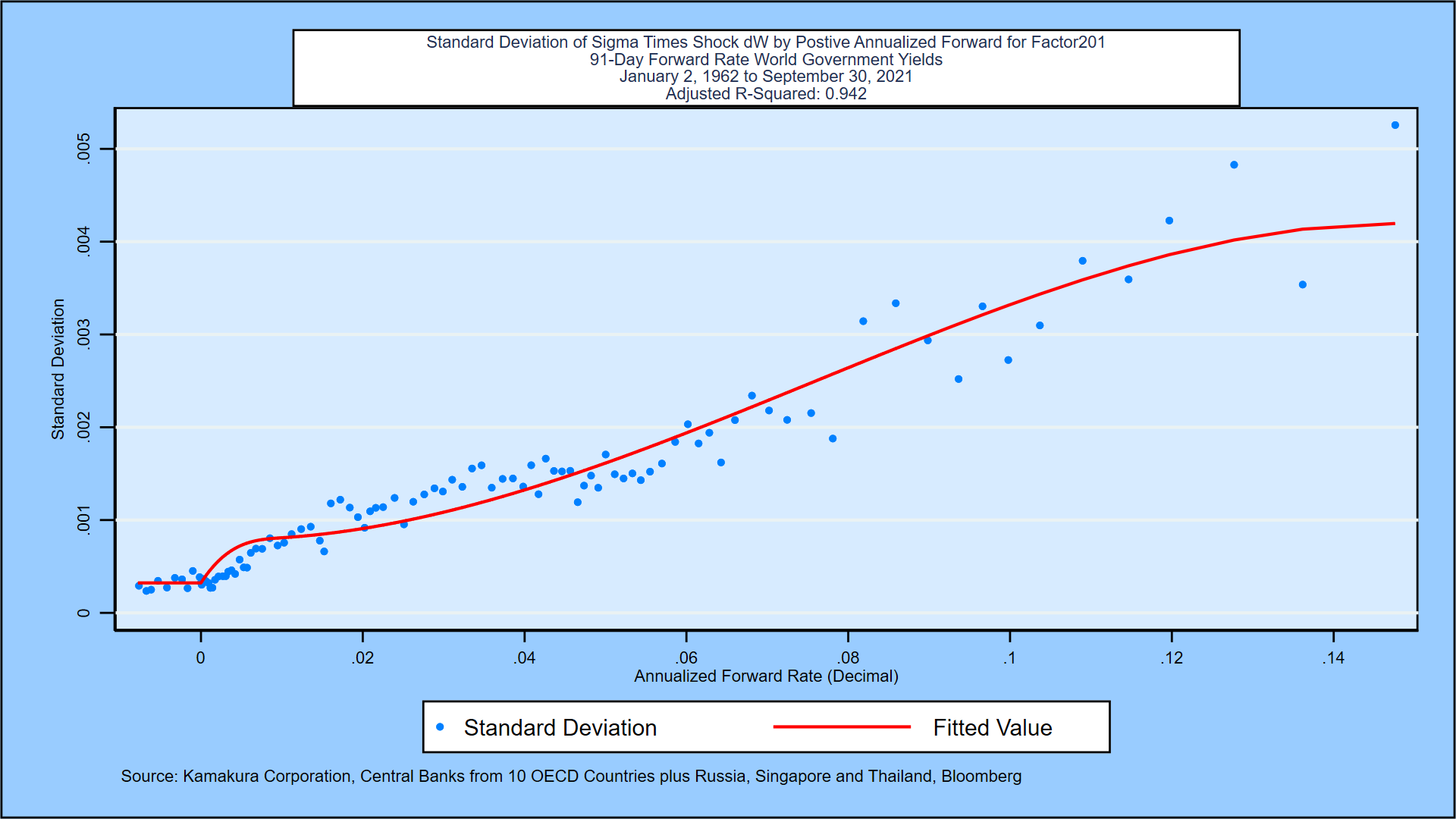
A 2-segment cubic spline of annualized forward rates explains 94.2%[2] of the variation in the standard deviation of forward rate changes for these ordered groups. This is the volatility function used when extracting the first random factor driving the 13-country yield curves. Note that the right-hand side of the curve has been constrained to have a first derivative of zero at a high level of rates.[3] The rise in volatility in higher rate environments has been confirmed in the government securities markets for each of the 13-country stand-alone data sets. Exhibit II shows the results for the second risk factor in the 13-country data set, the idiosyncratic movements in the 91-day forward rate maturing in 10 years:
Exhibit II
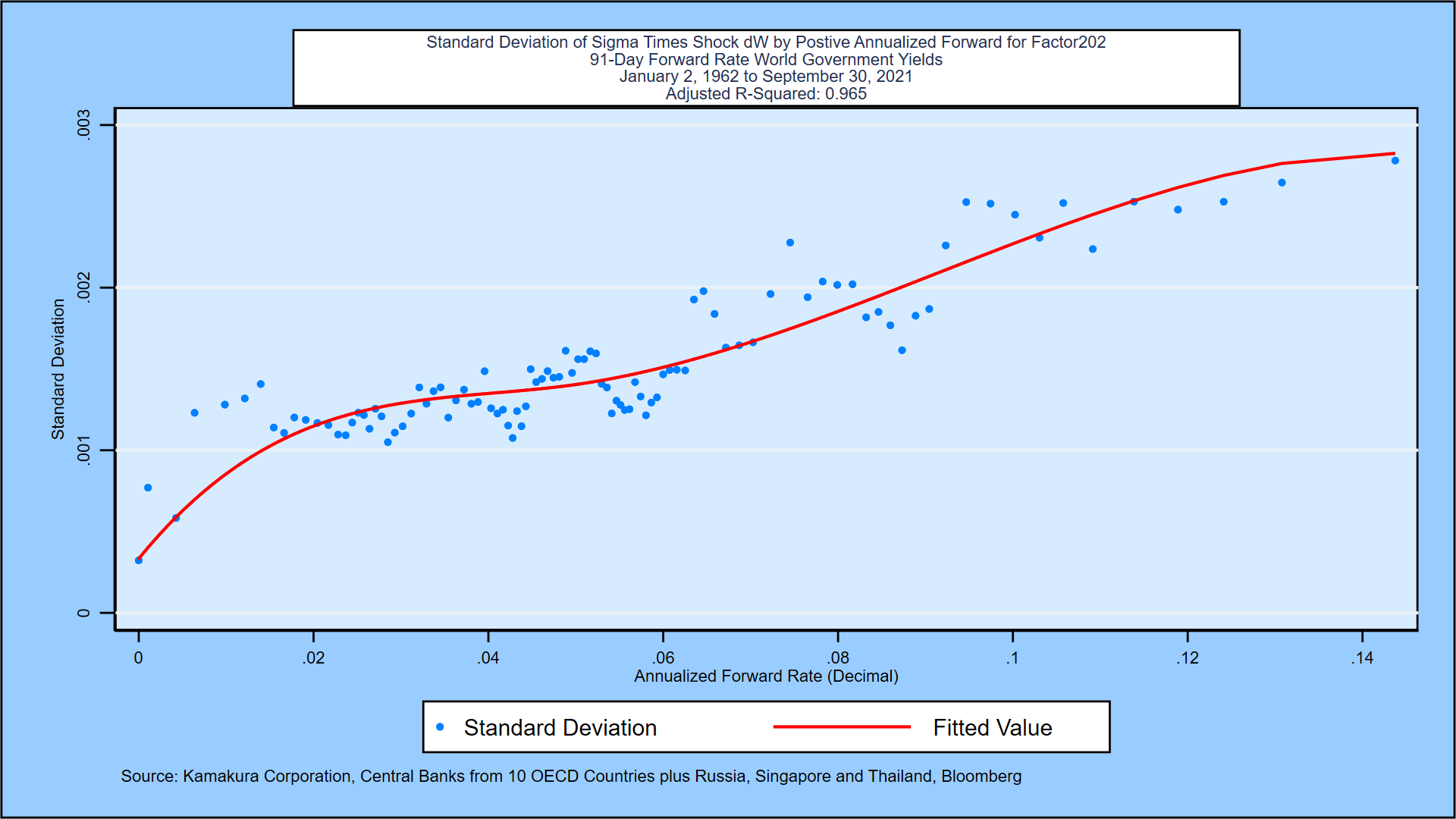
The cubic spline stochastic volatility specification explains 96.5% of the observed variation in forward rate volatility in the quarterly forward rate maturing at the 10-year point on the 13-country yield curves. We have imposed the same constraint on the first derivative and require that the fitted volatility not be less than the lowest observed volatility, which we discuss later in this section.
In Appendix C, we compare the span of the 13-country data set with the range of rates and maturities contained in certain of the 13-country stand-alone data sets. The U.S. data set spans 88.08% of the World experience, the highest amount among the 13 countries studied.
We use three statistical tests to determine whether or not the hypothesis of normality for forward rates and zero-coupon bond yields should be rejected at the 5% level: the Shapiro-Wilk test, the Shapiro-Francia test, and the skew test, all of which are available in common statistical packages. The 13-country history is now much larger than the maximum number of observations allowed by these tests. In early work, when the sample size was smaller, the hypothesis of normality was rejected at each 91-day forward rate maturity date for all 13 countries. We re-examine this hypothesis as needed using smaller samples from the full data set on a regular basis.
The rejection of the hypothesis of normality is problematic for constant coefficient or “affine” term structure models. In most of the other countries studied, the hypothesis of normality has been rejected strongly as well. Given these results, we proceed with caution on the implementation of the affine model.
In Chapter 3 of Advanced Financial Management (second edition, 2013), van Deventer, Imai and Mesler analyze the frequency with which U.S. Treasury forward rates move up together, down together or remain unchanged. This exercise informs the Heath, Jarrow, and Morton parameter fitting process and is helpful for the model validation questions posed in the Appendix. We perform the yield curve shift analysis using 90,720 days of quarterly forward rates for the 13-country consolidated yield curves. We analyze the daily shifts in the forward rates on each business day from January 2, 1962 through September 30, 2021. The results are given in Table II:
Table II
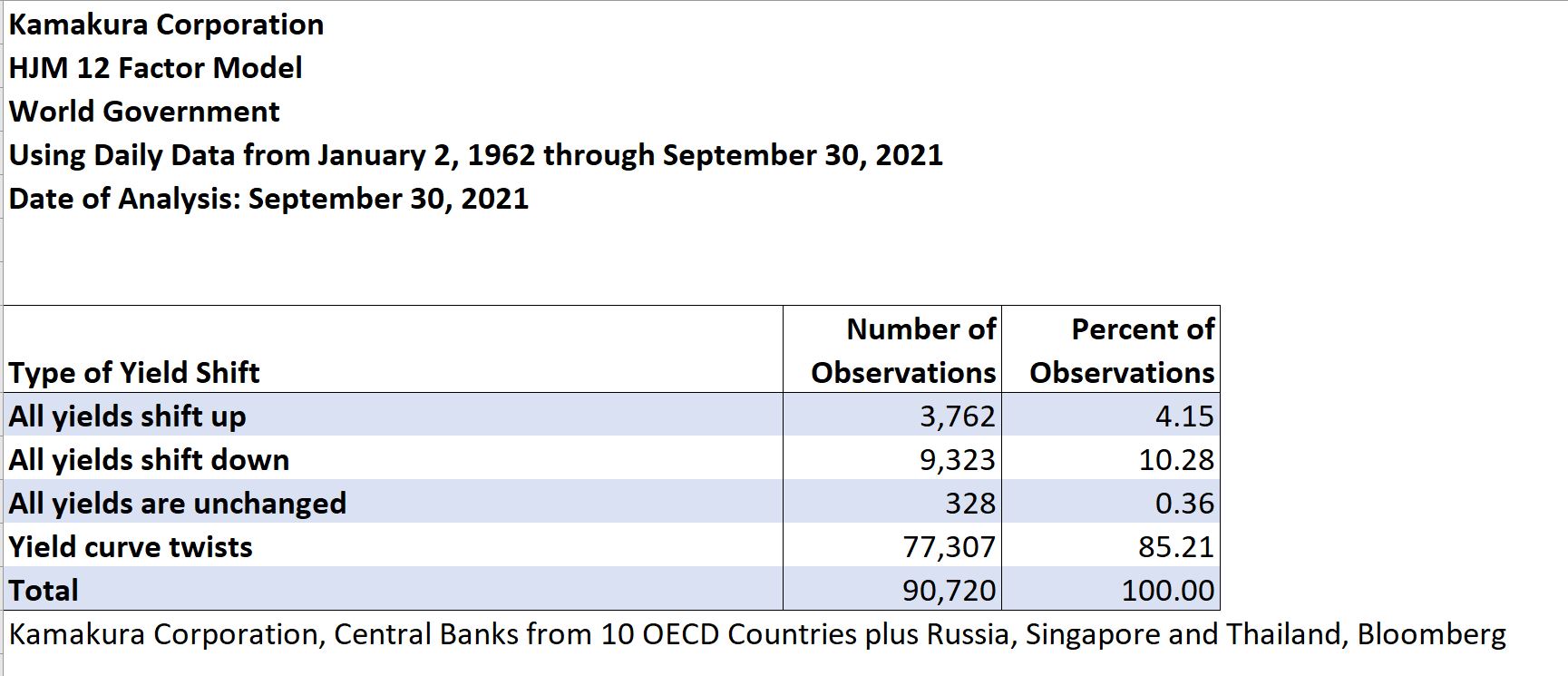
Yield curve shifts were all positive, all negative, or all zero 4.15%, 10.28%, and 0.36% of the time, a total of 14.79% of all business days. The predominant yield curve shift was a twist, with a mix of positive changes, negative changes, or zero changes. These figures are similar to those for the 13-country stand-alone data sets as well. These twists, which happen 85.21% of the time in the consolidated data base, cannot be modeled accurately with the conventional implementation of one-factor term structure models.
Another important aspect of yield curves is the number of local minima and maxima that have occurred over the modeling period. The results for the consolidated data set are given in Table III:
Table III
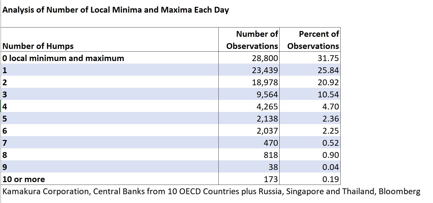
The number of days with 0 or 1 humps (defined as the sum of local minima and maxima on that day’s yield curve) was 57.59% of the total observations in the data set.
Finally, before proceeding, we count the number of occurrences of negative rates for each forward rate segment of the yield curve over the history provided by the consolidated data base.
Table IV

Table IV confirms that 91-day forward rates have been negative for approximately 5-10% of total observations for each of the first 12 forward rate segments. Rates have been negative for 12.044% of observations for 1-month yields in 13 countries over the same period, as shown in Appendix A.
Observed volatility in 1-month zero-coupon bond yields as a function of interest rate level for the standard 13-country World data set is shown in Exhibit III. Volatility trends upward as the yields at the beginning of the measurement period rise:
Exhibit III

III. Fitting Heath, Jarrow, and Morton Parameters
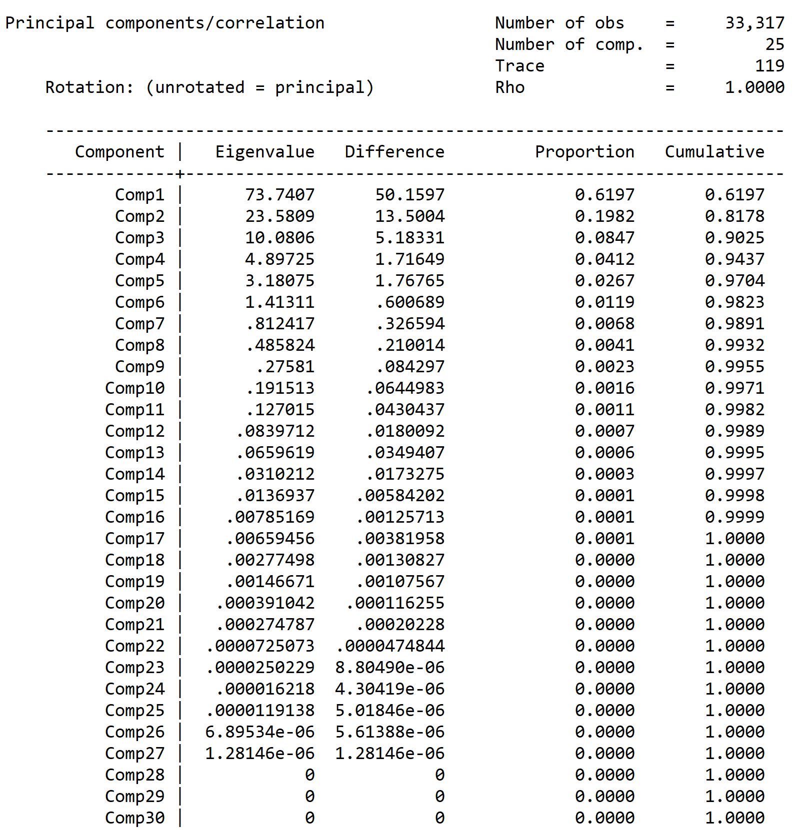
A simple first step in constructing a multi-factor Heath, Jarrow and Morton model is to conduct principal components analysis on the forward rates that make up the relevant yield curve. For the 13-country data set, at its longest maturity[4], these quarterly segments consist of one three-month spot rate and 119 forward rates. Over 33,317 observations, the principal components analysis indicates in Table V that the first factor explains only 61.97% of the movement in forward rates over the full curve. For a high degree of explanatory power, the principal components analysis indicates that 12 to 17 factors will be necessary.
Table V
With this analysis as background, we begin the Heath, Jarrow, and Morton fitting process.
In the studies done so far, the number of statistically significant factors are summarized below:
- Australia: Commonwealth Government Securities, 14 factors
- Canada: Government of Canada Securities, 7 factors
- France: French Government Bonds, 7 factors
- Germany: Bunds, 15 factors
- Italy: Italian Government Bonds, 11 factors
- Japan: Japanese Government Bonds, 8 factors
- Russia: Russian Government Bonds, 11 factors
- Singapore: Singapore Government Securities, 9 factors
- Spain: Spanish Government Securities, 11 factors
- Sweden: Swedish Government Securities, 11 factors
- Thailand: Thai Government Securities, 11 factors
- United Kingdom: Government Securities, 14 factors
- United States: Treasury Securities, 10 factors
- World: 13 countries’ government securities, prior version, 12 factors
We now fit a multi-factor Heath, Jarrow, and Morton model to the 13-country zero-coupon yield data from January 2, 1962 to September 30, 2021. For computational simplicity, we compress the data regimes numbered in the right-hand column of Table I to three regimes. The first is for observations where no maturity longer than 10 years was reported. The second is for those observations where no maturity longer than 20 years was reported. The third regime extends to the full 30-year maximum in the data set.
The procedures used to derive the parameters of a Heath, Jarrow and Morton model are described in detail in Jarrow and van Deventer (June 16, 2015 and May 5, 2017). We followed these steps to estimate the parameters of the model:
- We extract the zero-coupon yields and zero-coupon bond prices for all quarterly maturities out to 30 years for all daily observations for which the 30-year zero-coupon yield is available. For other observations, we extended the analysis to the longest maturity available, which varies by data regime. This is done using Kamakura Risk Manager, version 10.1, using the maximum smoothness forward rate approach to fill the quarterly maturity gaps in the zero-coupon bond data.
- We use overlapping 91-day intervals to measure changes in forward rates, avoiding the use of “quarterly” data because of the unequal lengths of calendar quarters. Because overlapping observations trigger auto-correlation, “HAC” (heteroscedasticity and autocorrelation consistent) standard errors are used. The methodology is that of Newey-West with 91-day lags.
- We consider twelve potential explanatory factors: the idiosyncratic portion of the movements in 91-day forward rates that mature in 6 months, 1 year, 1.5, 2, 3, 5, 7, 10, 15, 20, 25, and 30 years.
- We calculate the discrete changes in forward returns as described in the parameter technical guide. Because the discrete changes are non-linear in the no-arbitrage framework of Heath, Jarrow, and Morton, we use generalized linear models and the proper HJM functional form to fit interest rate volatility.
- We use a different non-linear regression for each segment of the yield curve. We considered a panel-based approach, but we rejected it for two reasons: first, the movement of parameters as maturity lengthens is complex and not easily predictable before estimation; second, the residual unexplained error in forward rates is very, very small, so the incremental merit of the panel approach is minimal.
- We then begin the process of creating the orthogonalized risk factors that drive interest rates using the Gram-Schmidt procedure. These factors are assumed, without loss of generality, to be uncorrelated independent random variables that have a normal distribution with mean zero and standard deviation of 1.
- Because interest volatility is assumed to be stochastic, simulated out-of-sample forward rates will not in general be normally distributed. We also calculate constant volatility parameters and choose the most accurate from the constant volatility and stochastic volatility models estimated.
- In the estimation process, we added factors to the model as long as each new factor provided incremental explanatory power. The standard suite of models in both cases includes 1 factor, 2 factors, 3 factors, 6 factors and “all factors,” which varies by country.
We postulate that unannualized interest rate volatility for each forward rate maturity k is a cubic function of the annualized forward rate that prevails for the relevant risk factor j at the beginning of each 91-day period:

When the initial forward rate is negative, we postulate that interest rate volatility is a constant[5]. Using Japan volatility data, the measured b0,jk was 0.1408%. Using the 13-country World model, the value of b0,jk is 0.0478%.
We use the resulting parameters and accuracy tests to address the hypothesis that a one-factor model is “good enough” for modeling 13-country government yields in Appendix A. We report the accuracy results for 1, 2, 3, 6 and all (12) factors. The factors are the idiosyncratic variation in 91-day forward rates at each of 12 maturities. The factors, described by the maturity of the quarterly forward rate used, are added to the model in this order:
- Data Regime 1 (Maturities of 10 years or less)
- Factor 1: 6 months
- Factor 2: 10 years
- Factor 3: 3 years
- Factor 4: 7 years
- Factor 5: 1 year
- Factor 6: 5 years
- Factor 7: 2 years
- Factor 8: 5 years
- Data Regime 2 (Maturities longer than 10 years up to 20 years)
- Factor 9: 15 years
- Factor 10: 20 years
- Data Regime 3 (Maturities longer than 20 years up to 30 years)
- Factor 11: 25 years
- Factor 12: 30 years
Exhibit IV summarizes the adjusted r-squared for the non-linear equations for each of the 119 quarterly forward rate segments that make up the 13-country yield curves:
Exhibit IV

The adjusted r-squared for the best practice model over each of the forward rates is plotted in blue and is near 100% for all 119 quarterly segments of the yield curve. The one-factor model in red, by contrast, does a poor job of fitting 91-day movements in the quarterly forward rates. The adjusted r-squared is good, of course, for the first forward rate since the short rate is the standard risk factor in a one-factor term structure model. Beyond the first quarter, however, explanatory power declines rapidly. The adjusted r-squared of the one-factor model never exceeds 20% after the first 17 quarterly forward rates and is below that level at most maturities.
The root mean squared error for the 1, 2, 3, 6 and all (12) factor stochastic volatility models is shown in Exhibit V.
Exhibit V

The root mean squared error for the 12-factor model is less than 0.05% at every maturity along the yield curve. This result should not come as a surprise to a serious analyst, because it is very similar to the results of the best practice Heath, Jarrow, and Morton term structure models for each the 13 government bond markets studied on a stand-alone basis.
Bayesian Considerations in Model Validation
Kamakura term structure model validation is conducted in the spirit of Bayesian iterative model building as outlined by Gelman et al. This quote[6] from Gelman et al [2013] explains the Bayesian estimation process:
“The process of Bayesian data analysis can be idealized by dividing it into the following three steps:
- Setting up a full probability model—a joint probability distribution for all observable and unobservable quantities in a problem. The model should be consistent with knowledge about the underlying scientific problem and the data collection process.
- Conditioning on the observed data: calculating and interpreting the appropriate posterior distribution—the conditional probability distribution of the unobserved quantities of ultimate interest, given the observed data.
- Evaluating the fit of the model and the implications of the resulting posterior distribution: how well does the model fit the data, are the substantive conclusions reasonable, and how sensitive are the results to the modeling assumptions in step 1? In response, one can alter or expand the model and repeat the three steps.”
Jarrow and van Deventer go on to explain that the iterative process described above by Gelman et al is especially important in fitting Heath, Jarrow, and Morton parameters for the following reasons:
- Negative interest rates have been observed in Japan, Hong Kong, and many European countries, but many other countries, including the U.S., have yet to experience negative rates. In the U.S. case, the U.S. Department of the Treasury notes on its website that it overrides observed negative yields in the market with zero values.
- The “knowledge about the underlying scientific problem” from the historical data available is as follows: (1) negative rates are possible, (2) they are much less likely to occur than positive rates, (3) interest rate volatility that results when rates are negative is of high interest but the historical data is either limited or non-existent, depending on the country, and (4) an international data set would best shed light on this and other HJM issues.
There are other issues relevant to estimation:
- As noted by Heath, Jarrow, and Morton [1992], stochastic volatility driven by interest rate levels must be capped to avoid a positive probability of infinitely high interest rates.
- Subject to this cap, most market participants expect interest rate volatility to rise as rates rise and that the interest rate volatility that prevails when rates are negative represents the lowest level of volatility that would prevail. Historical experience with negative rates so far around the world makes it clear that interest rate volatility does not go to zero at any rate level.
- Most market participants believe that the empirical drift in forward rates that occurs (i.e., the change in observed empirical interest rates in the case where all interest rate shocks are zero) varies by the level of interest rates. The stochastic volatility model described in this paper assumes that empirical drift is a cubic function of annualized forward rates.
To summarize, a model validation effort in the Bayesian spirit would address at least these issues:
- Tests of smoothness of simulated curves
- Tests to confirm existence of negative rates in selected circumstances in the simulation
- Comparison of simulated risk neutral and empirical yields
- Time series distribution of simulated risk neutral and empirical yields
- Tests for the reasonableness of empirical drift in rates at each segment of the yield curve and stress tests of the rate factor volatility functions for reasonableness over the full range of rates that have been observed in the past. These tests are shown in Appendix B
We conduct an inspection of these issues with the aid of a forward-looking out-of-sample simulation of U.S. Treasury yields from a starting point of October 15, 2021 using both the World term structure model coefficients and the U.S. single-country model coefficients with the following specifications:
- Yield curve: U.S. Treasury yields
- Date of yields: October 15, 2021
- Number of scenarios: 500,000
- Simulation time horizon: 30 years
- Simulation periodicity: 91 days (quarterly)
Smoothness Validation
First, we select a random sample of 10 scenarios at each time step and visually examine them for smoothness. We can also use the discrete formula for smoothness given above to identify any outliers and examine the scenarios in question. These graphs provide informal confirmation that nothing in the model estimation procedure has introduced artificial lumpiness in the simulated yield curves. A quantitative assessment of the smoothness of all 500,000 yield curves at each time step would provide the more formal confirmation that the yield curves simulated are realistically smooth. For samples of the graphics used, please contact the author via info@kamakuraco.com.
Distribution of Simulated Risk Neutral and Empirical Rates
We now examine the probability distributions of empirical simulated rates at various maturities over time. We seek to detect visually any points in time at which the simulated distribution of yields is strange or unrealistic. In the following exhibits, we focus on three-month U.S. Treasury yields for both the World and U.S.-only models:
Exhibit VI: Three-Month U.S. Treasury Yields at 1 Year

The U.S. only model is denoted the base model and shown in blue. The World or “comparison” model, is shown in red. The World model at a 1-year horizon shows less volatility in simulated empirical 3-month Treasury bill yields.
Exhibit VII: Three-Month U.S. Treasury Yields at 5 Years

By the 5-year point in the simulation, the red bars of the World model show a higher level of negative observations and are visibly skewed to the left compared to the U.S.-only base model. This pattern continues through the 10-year and 15-year time horizons.
Exhibit VIII: Three-Month U.S. Treasury Yields at 10 Years

At the 10-year point in the simulation, World model empirical 3-month yields continue to show more negative observations and lower volatility than the U.S.-only model.
Exhibit IX: Three-Month U.S. Treasury Yields at 15 Years

The pattern of previous Exhibits continues, as the World model at 15 years has significantly more negative rate observations and a tighter distribution than that generated from the U.S.-only model.
The simulated distribution of empirical 3-month rates shows the richness of the empirical drift function employed in both the World and U.S.-only HJM model. We stress test the derived coefficients in the Appendices.
Time Series Distribution of Simulated Yields
We also plot the time series graphs of the mean, median, high, low, and various percentiles for empirical rates. We again seek to determine that there are no unexpected variations in the distribution of empirical yields over time. We can confirm that there are no unexpected variations in the distribution of empirical yields over time.
Simulation of the Term Premium
The size of the “term premium” of actual zero-coupon yields over the expected level of the short rate is a topic of great interest to both academics and policy makers. In a stochastic volatility model, the term premium must be determined by simulation because in general there is no closed-form solution for expected future rates. Exhibit X shows a much wider term premium for the U.S. using the World coefficients. The term premium widens significantly initially, and then it widens at a slower pace over longer maturities.
Exhibit X: Simulation of the Term Premium
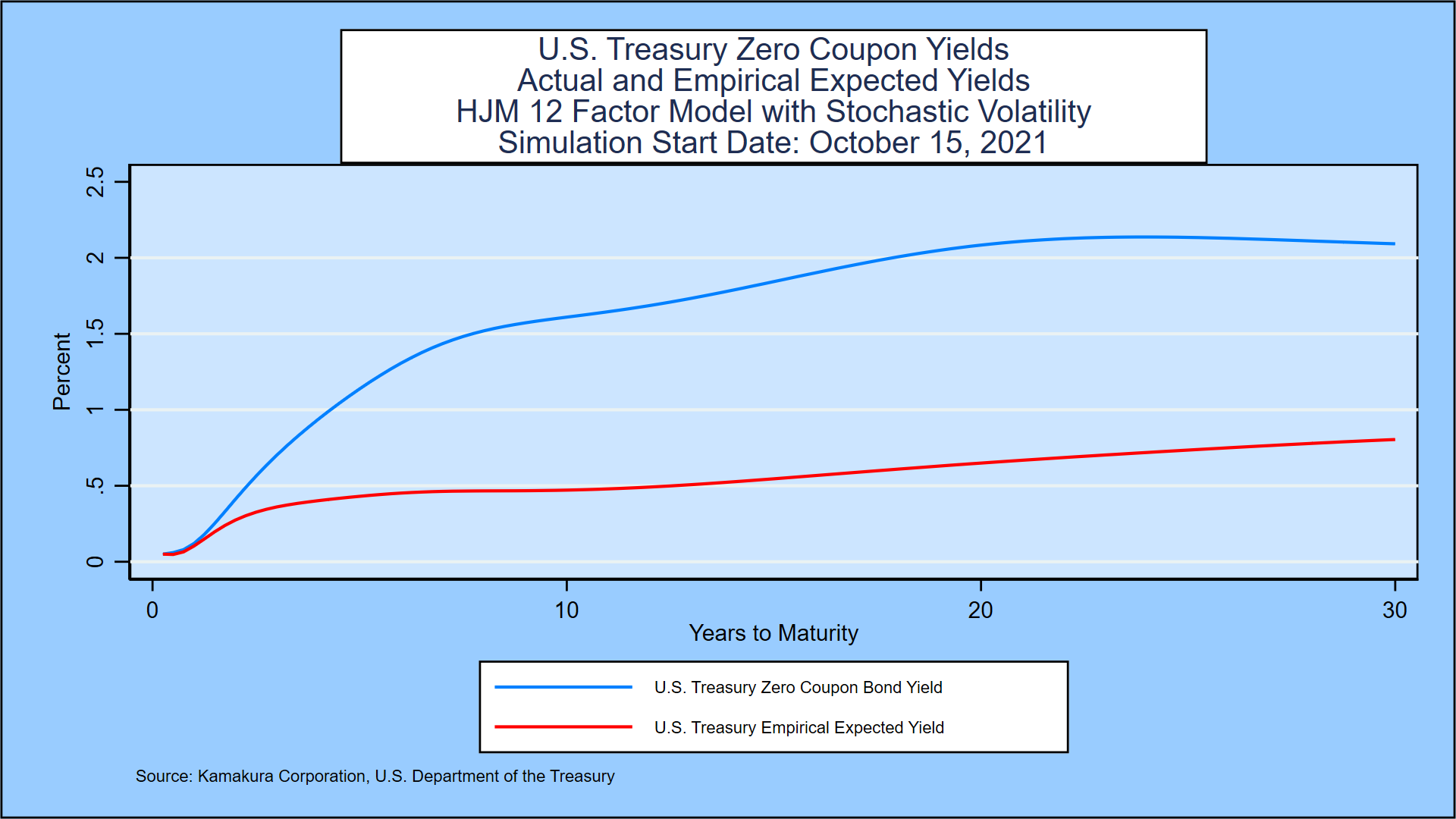
We again conclude that the simulation produces results that are consistent with the “scientific knowledge” about the variation in interest rates around the world.
Probability of Negative Short-term Interest Rates
Exhibit XI shows the simulated probability of negative empirical 3-month Treasury bill rates at each 91-day time step using the World coefficients. Because of the sharp increase in forward rates embedded in the October 15, 2021 yield curve, the probability of negative rates drops initially and then rises to a level significantly above the probabilities generated using U.S.-only term structure model parameters.
Exhibit XI

IV. Conclusion
The 13-country government yield curves are driven by 12 factors, a number of factors very similar to the average for the single-country government yield studies.
The stochastic volatility assumption provides more accurate and more reasonable parameters than a constant volatility model, particularly in the context of Bayesian simulations as part of the model validation process. Exhibit XII summarizes the reasons for those conclusions:
Exhibit XII: Statistical Significance Summary and Volatility Classification
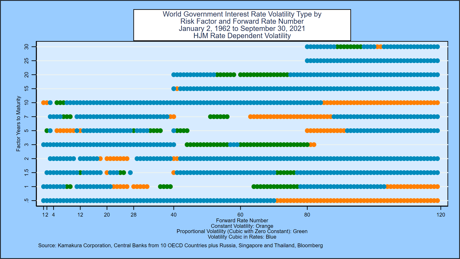
The vertical axis lists the maturities used as risk factors by years to maturity of the underlying quarterly forward rate. The risk factors are the idiosyncratic movement of each of these forward rates. If the risk factor is statistically significant in explaining the movement of forward rates with the quarterly maturities listed on the horizontal axis, a dot is placed in the grid. Note that the quarterly forward rates maturing in 15 and 20 years are only used as explanatory variables for maturities from 10 to 30 years. Similarly, the 25 and 30-year factors are used only for maturities over 20 years.
The nature of interest rate volatility for each combination of risk factor maturity and forward rate maturity is color coded. If the derived volatility is constant, the color code is orange. This is the affine specification. The graph shows immediately that a small minority of the risk factor maturity/forward rate maturity volatilities is consistent with the affine structure. The green and blue codes address the issue of whether interest rate volatility for that combination of risk factor maturity and forward rate maturity is zero or not when the forward rate is zero. If the measured volatility at a zero forward rate level is zero, the color code is green. Otherwise, the color code is blue. In both cases, the volatility is a stochastic function of the forward rates at the start of the simulation period.
The chart summarizes the fact that all 12 factors are statistically significant across the yield curve for the 13-country data set. The dominant derived interest rate volatility is the cubic stochastic volatility specification with a non-zero constant. An affine assumption for interest rate volatility is best fitting for a small minority of the combinations of risk factor maturity and forward rate maturity.
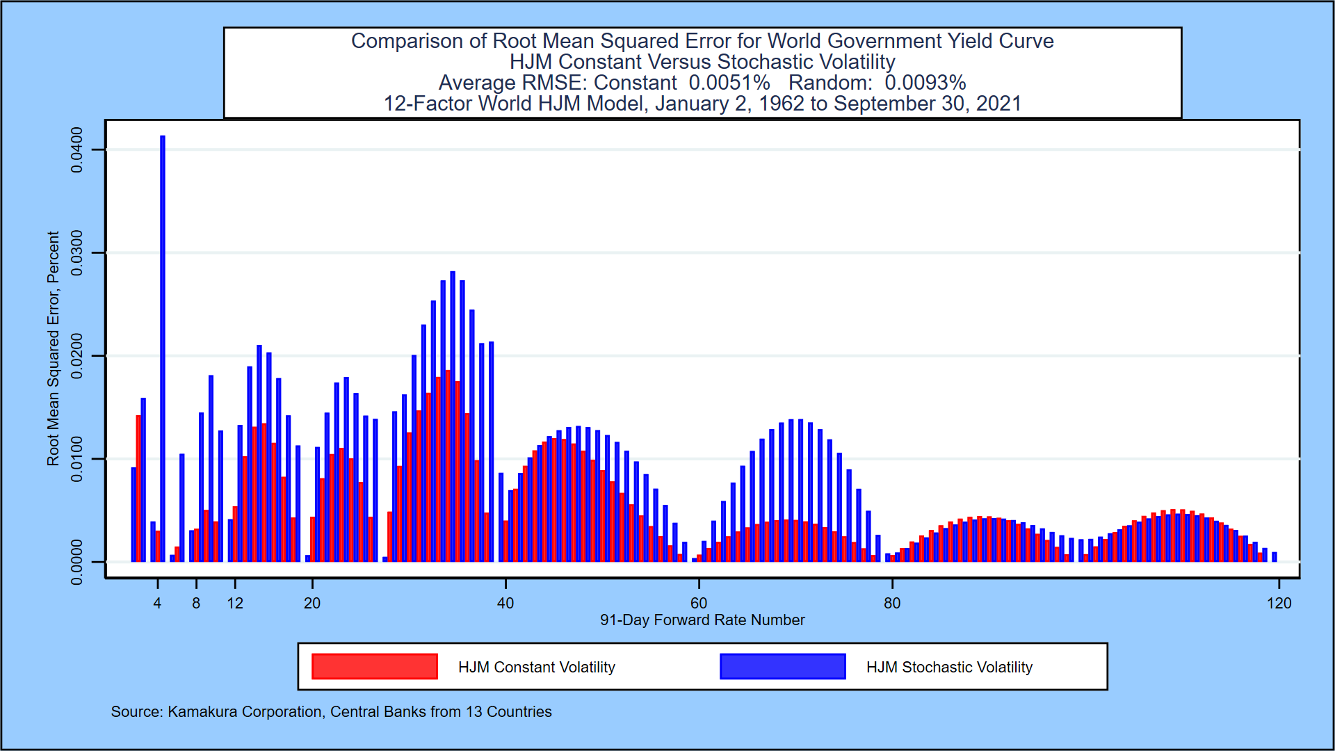
That being said, Exhibit XIII shows that the average root mean squared error for a 12-factor constant coefficient model is slightly below the average root mean squared error for the stochastic volatility model. Additional research on this point is forthcoming in subsequent editions of this paper.
Exhibit XIII: Root Mean Squared Error Comparison
Appendix A: Single-Factor versus Multiple-Factor Models
In spite of the overwhelming evidence across countries that government bond yields are driven by multiple factors, the use of single-factor term structure models in interest rate risk management systems remains common even in some of the world’s largest banks. This appendix asks and answers a number of important questions on the use of one- factor models that any sophisticated model audit would pose. Given the answers below, most analysts would conclude that one-factor term structure models are less accurate than a long list of multi-factor term structure models and that the one-factor models would therefore fail a model audit.
We address two classes of one-factor term structure models, all of which are special cases of the Heath, Jarrow, and Morton framework, in this appendix using data from the 13-country data set.
- One-factor models with rate-dependent interest rate volatility:
- Cox, Ingersoll, and Ross (1985)
- Black, Derman and Toy (1990)
- Black and Karasinski (1991)
- One-factor models with constant interest rate volatility (affine models):
- Vasicek (1977)
- Ho and Lee (1986)
- Extended Vasicek or Hull and White Model (1990, 1993)
Non-parametric test 1: Can interest rates be negative in the model?
The one-factor models with rate-dependent interest rate volatility make it impossible for interest rates to be negative without ad hoc shifts in the simulated yield curves. Is this implication true or false? It is false, as this histogram of 1-year zero-coupon bond yields from government securities in 13 countries confirms. 10.280% of observations were negative:
Exhibit A1

Non-parametric test 2: As commonly implemented, one-factor term structure models imply that all yields will either (a) rise, (b) fall, or (c) remain unchanged. This implication is false, as documented for the 13-country data set in Table II. In fact, yield curves have twisted on 85.21% of the observations for the World government markets studied.
Non-parametric test 3: The constant coefficient one-factor models imply that zero-coupon yields are normally distributed and so are the changes in zero-coupon yields. In each of the 13 individual country studies, this implication is rejected by three common statistical tests for 120 of 120 quarterly maturities for zero yields and for all 120 of the quarterly changes. This histogram of 1-month zero-coupon bond yields from consolidated zero-coupon bond yields in 13 countries provides simple visual confirmation that normality is a poor approximation to the probability distribution of interest rates.
Exhibit A2

Assertion A: There are no factors other than the short-term rate of interest that are statistically significant in explaining yield curve movements.
This assertion is false. Table V shows, using principal components analysis, that 12-17 factors are needed to explain the movements of the 13-country yield dataset. Exhibit XII makes the same point in more detail.
Assertion B: There may be more than one factor, but the incremental explanatory power of the 2nd and other factors is so miniscule as to be useless.
This assertion is false, as the 2nd through 12th factors in the 13-country data set explain 38.03% of forward rate movements, compared to 61.97% for the first factor alone. In most countries, the best “first factor” is not the short rate of interest used by many large banks; it is the parallel shift factor of the Ho and Lee model.
Assertion C: A one-factor “regime shift” model is all that is necessary to match the explanatory power of the 2nd and other factors.
This assertion is also false. A recent study prepared for a major U.S. bank regulator also confirmed that a one-factor “regime shift” term structure model made essentially no incremental contribution toward resolving the persistent lack of accuracy in one-factor term structure models.
Finally, a Kamakura Corporation study comparing a 1-factor and 10-factor Heath Jarrow and Morton simulation results shows that the simulated volatility of interest rates is underestimated by 61% to 83% in the one-factor model. Moreover, the average level of simulated U.S. Treasury yields is biased lower. Finally, the probability of negative rates implied by the one-factor model is also biased low as shown here:
Table A1

Appendix B: Tests of Empirical Drift and Stress Tests of Rate Volatility
A determination that out-of-sample simulations will be “consistent with scientific knowledge of the problem” can in fact be gleaned without a full simulation. One practical modeling objective is to obtain out-of-sample rate scenarios that “do not blow up,” rising or falling to extreme values that are highly unlikely to occur in reality. Heath, Jarrow, and Morton make it clear how this objective is achieved in an HJM model:
- First of all, rate shocks and rate volatilities are the same for the simulation of both risk neutral and empirical rates.
- This requires that the interest rate volatility functions be capped to prevent “explosions” in rate simulations, as we have done above.
- HJM also make it clear that the risk neutral drift in each segment of the yield curve is completely determined by the choice of volatility functions and the slope of the initial yield curve. This insight is not apparent to many practitioners because the early work of Vasicek [1977] and Hull and White 3 decades ago seems to embed mean reversion in risk neutral interest rates.
- The drift in empirical rates, however, is determined econometrically. In the model above the drift function employed adds a cubic function of the corresponding forward rate to the base drift that applies when rates are zero or below.
The Bayesian “scientific knowledge” of empirical rate movements leads us to expect some mean reversion in rates. When rates are high, we expect the empirical drift will be negative in each section of the empirical yield curve. When rates are low, we expect that the empirical drift to be positive. By applying hypothetical flat yield curves from zero (or less) to 15%, we can confirm that empirical drift in the U.S. Treasury stand-alone HJM model is consistent with these expectations.
Exhibit B1

The empirical drift for the World model through September 30, 2021 is shown in Exhibit B2.
Exhibit B2

Simply by visual inspection, it is clear that the fitted drift in empirical rates for the World model shows mean reversion that is reasonably similar to that fitted to U.S. data alone.
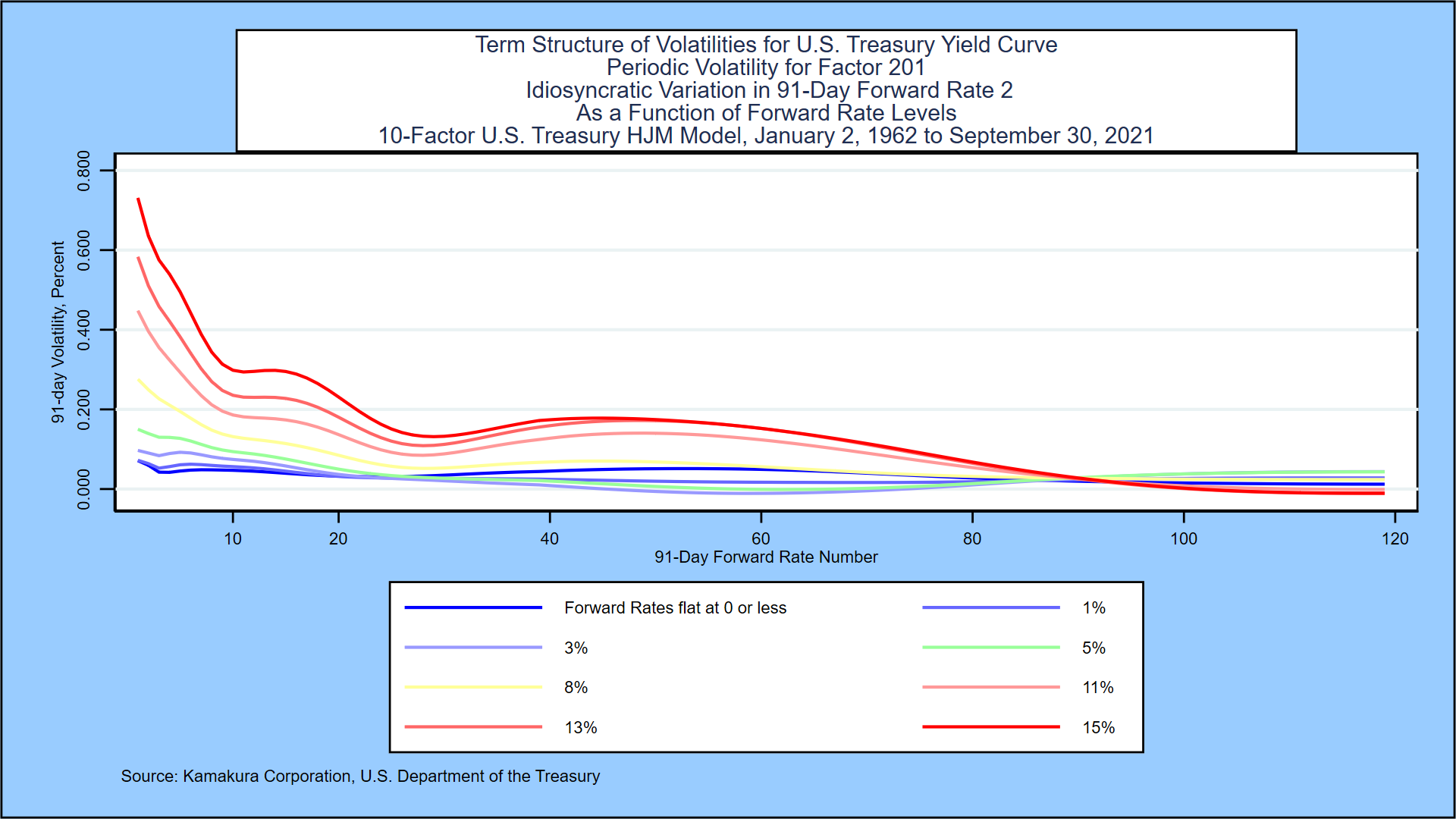
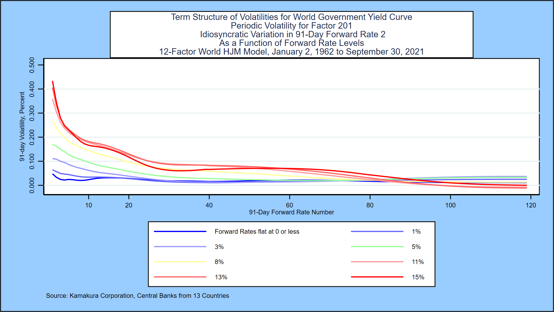
We can apply the same tests to the interest rate volatility functions to confirm their robustness and that they do not “blow up” at either very high or very low-rate levels. The first factor in the model above is the idiosyncratic movement in the first random forward rate segment. We expect this first factor to have volatility that declines with maturity, and which is higher when rates are high. The graph below shows that those expectations are met by U.S. Treasury single-country data:
Exhibit B3
We again compare the U.S. stand-alone model movements in interest rate volatility for the first factor with World experience, shown in Exhibit B4:
Exhibit B4
The World interest rate volatility again shows a stress-tested pattern that is both similar to U.S. data alone and consistent with expectations.
The second factor in the model is the idiosyncratic variation in the 91-day forward rate segment maturing in 10 years. Because this point is near the middle of the yield curve, we expect volatility functions can be both positive and negative. Our main concern is that volatility does not blow up as we stress test the level of the forward rate curve. Again, our expectations are met, as shown below for the U.S. stand-alone model.
Exhibit B5

How does this compare with volatility for the second factor (which is also the idiosyncratic movements in the 91-day forward rate maturing in 10 years) for the World model? The answer is given in Exhibit B6:
Exhibit B6

Here, the results of the World model differ from the U.S.-only model. An upward shock in the 10-year forward rate drives up yields in the middle of the World yield curve, with smaller impacts on the short end and long end of the curve. Generally speaking, volatility increases as the level of the 10-year forward rate rises. This pattern is more consistent with the author’s expectations than the U.S.-only results.
Appendix C: Comparing the Span of Interest Rates with the World Data Set
A common econometric challenge is fitting a model to the data at hand and measuring the risk that the model behaves badly out of sample. One measure of this risk for each single-country data set is to compare the range of interest rates experienced with the consolidated13-country World data set over maturities to 30 years. We use monthly zero-coupon bond yields for these calculations. The results are shown in Exhibit C1 for the U.S. stand-alone data set and the consolidated World data set:
Exhibit C1

The U.S. data set spans 88.08% of World interest rate experience. This is the highest proportion of any of the 13 countries included in the World data set. Even in the U.S. case, however, using the coefficients of the World model would provide greater realism in simulations when rates turn negative than a stand-alone U.S. model and perhaps more realistic responses of volatility to forward rates levels as we saw in Exhibits VI to IX.
REFERENCES
Adams, Kenneth J., and Donald R. van Deventer, “Fitting Yield Curves and Forward Rate Curves with Maximum Smoothness,” Journal of Fixed Income, 1994, pp. 52-61.
Adrian, Tobias, Richard K. Crump and Emanuel Moench, “Pricing the Term Structure with Linear Regressions,” Federal Reserve Bank of New York, Staff Report 340, August 2008, revised August 2013.
Angrist, Joshua D. and Jorn-Steffen Pischke, Mostly Harmless Econometrics: An Empiricist’s Companion, Princeton University Press, Princeton, 2009.
Berger, James O. Statistical Decision Theory and Bayesian Analysis, second edition, Springer-Verlag, 1985.
Berry, Donald A. Statistics: A Bayesian Perspective, Wadsworth Publishing Company, 1996.
Campbell, John Y, Andrew W. Lo, and A. Craig McKinley, The Econometrics of Financial Markets, Princeton University Press, 1997.
Gelman, Andrew and John B. Carlin, Hal S. Stern, David B. Dunson, Aki Vehtari, and Donald B. Rubin, Bayesian Data Analysis, third edition, CRC Press, 2013.
Goldberger, Arthur S. A Course in Econometrics, Harvard University Press, 1991.
Hamilton, James D. Times Series Analysis, Princeton University Press, 1994.
Hansen, Bruce E. Econometrics, University of Wisconsin, January 15, 2015.
Hardin, James W., and Joseph M. Hilbe, Generalized Linear Models and Extensions, fourth edition, Stata Press, College Station, Texas, 2018.
Hastie, Trevor, Robert Tibshirani and Jerome Friedman, Elements of Statistical Learning: Data Mining, Inference and Prediction, Springer, second edition, tenth printing, 2013.
Heath, David, Robert A. Jarrow, and Andrew Morton, “Bond Pricing and the Term Structure of Interest Rates: A Discrete Time Approach,” Journal of Financial and Quantitative Analysis, 1990, pp. 419-440.
Heath, David, Robert A. Jarrow, and Andrew Morton, “Contingent Claims Valuation with a Random Evolution of Interest Rates,” The Review of Futures Markets, 9 (1), 1990, pp. 54 -76.
Heath, David, Robert A. Jarrow, and Andrew Morton,” Bond Pricing and the Term Structure of Interest Rates: A New Methodology for Contingent Claim Valuation,” Econometrica, 60(1),1992, pp. 77-105.
Heath, David, Robert A. Jarrow, and Andrew Morton, “Easier Done than Said”, RISK Magazine, October 1992.
Jarrow, Robert A. Modeling Fixed Income Securities, and Interest Rate Options, second edition, Stanford University Press, Stanford, 2002.
Jarrow, Robert A. and Stuart Turnbull, Derivative Securities, second edition, South-Western College Publishing, Cincinnati, 2000.
Jarrow, Robert A., and Donald R. van Deventer, “Monte Carlo Simulation in a Multi-Factor Heath, Jarrow and Morton Term Structure Model,” Kamakura Corporation Technical Guide, Version 4.0, June 16, 2015
Jarrow, Robert A., and Donald R. van Deventer, “Parameter Estimation for Heath, Jarrow and Morton Term Structure Models,” Kamakura Corporation Technical Guide, Version 4.0, May 5, 2017.
Johnston, J. Econometric Methods, McGraw-Hill, 1972
Kim, Don H., and Jonathan H. Wright, “An Arbitrage-Free Three Factor Term Structure Model and the Recent Behavior of Long-Term Yields and Distant-Horizon Forward Rates,” Finance and Economics Discussion Series, Federal Reserve Board, 2005-33.
Maddala, G. S. Introduction to Econometrics, third edition, John Wiley & Sons, 2005.
Papke, Leslie E. and Jeffrey M. Wooldridge, “Econometric Methods for Fractional Response Variables with an Application to 401(K) Plan Participation Rates,” Journal of Applied Econometrics, Volume 11, 619-632, 1996.
Robert, Christian P. The Bayesian Choice: From Decision-Theoretic Foundations to Computational Implementation, second edition, Springer Science+Business Media LLC, 2007.
Stock, James H. and Mark W. Watson, Introduction to Econometrics, third edition, Pearson/Addison Wesley, 2015.
Studenmund, A. H. Using Econometrics: A Practical Guide, Addison-Wesley Educational Publishers, 1997.
Theil, Henri. Principles of Econometrics, John Wiley & Sons, 1971.
van Deventer, Donald R. “Interest Rate Risk: Lessons from 2 Decades of Low Interest Rates in Japan,” Kamakura Corporation working paper, www.kamakuraco.com, August 11, 2016.
van Deventer, Donald R. “A Multi-Factor Heath Jarrow and Morton Model of the Australia Commonwealth Government Securities Yield Curve,” Kamakura Corporation working paper, www.kamakuraco.com, August 27, 2015.
van Deventer, Donald R. “A Multi-Factor Heath Jarrow and Morton Model of the Swedish Government Bond Yield Curve,” Kamakura Corporation working paper, www.kamakuraco.com, September 3, 2015.
van Deventer, Donald R. “Spanish Government Bond Yields: A Multi-Factor Heath Jarrow and Morton Model,” Kamakura Corporation working paper, www.kamakuraco.com, September 10, 2015.
van Deventer, Donald R. “Singapore Government Securities Yields: A Multi-Factor Heath Jarrow and Morton Model,” Kamakura Corporation working paper, www.kamakuraco.com, September 22, 2015.
van Deventer, Donald R. “The Regime Change Term Structure Model: A Simple Model Validation Approach,” Kamakura Corporation working paper, www.kamakuraco.com, January 26, 2016.
van Deventer, Donald R. “An 8 Factor Heath, Jarrow and Morton Model for the Japanese Government Bond Yield Curve, 1974 to 2016: The Impact of Negative Rates and Smoothing Issues,” Kamakura Corporation working paper, www.kamakuraco.com, June 21, 2017.
van Deventer, Donald R. “A 10-Factor Heath, Jarrow, and Morton Stochastic Volatility Model for the U.S. Treasury Yield Curve, Using Daily Data from January 1, 1962 through June 30, 2021.” Kamakura Corporation working paper, www.kamakuraco.com, July 19, 2021.
van Deventer, Donald R. “A 7-Factor Heath, Jarrow and Morton Stochastic Volatility Model for the Government of Canada Yield Curve, Using Daily Data from January 2, 2001 to August 31, 2021.” Kamakura Corporation working paper, www.kamakuraco.com, September 22, 2021.
van Deventer, Donald R. “An 11-Factor Heath, Jarrow, and Morton Stochastic Volatility Model for the Government of Russia Yield Curve Using Daily Data from January 4, 2003 through August 31, 2021,” Kamakura Corporation working paper, www.kamakuraco.com, September 30, 2021.
van Deventer, Donald R. “A 15-Factor Heath, Jarrow, and Morton Stochastic Volatility Model for the German Bund Yield Curve, Using Daily Data from August 7, 1997 through September 30, 2021,” Kamakura Corporation working paper, www.kamakuraco.com, October 6, 2021.
van Deventer, Donald R. “A 10-Factor Heath, Jarrow, and Morton Stochastic Volatility Model for the U.S. Treasury Yield Curve, Using Daily Data from January 1, 1962 through September 30, 2021,” Kamakura Corporation working paper, www.kamakuraco.com, October 13, 2021.
van Deventer, Donald R., Kenji Imai and Mark Mesler, Advanced Financial Risk Management, second edition, John Wiley & Sons, Singapore, 2013.
Woolridge, Jeffrey M. Econometric Analysis of Cross Section and Panel Data, The MIT Press, 2002.
Footnotes
[1] Kamakura Corporation, 2222 Kalakaua Avenue, Suite 1400, Honolulu, Hawaii, USA, 96815. E-Mail dvandeventer@kamakuraco.com. The author wishes to thank Prof. Robert A. Jarrow for 27 years of conversations on this topic. Daniel Dickler, Theodore Spradlin, and Dr. Xiaoming Wang provided invaluable data services and smoothing analysis using Kamakura Risk Manager. The author also wishes to thank the participants at seminars organized by the Bank of Japan and the Federal Reserve Bank of San Francisco at which papers addressing similar issues were presented.
[2] Note that the simple r-squared is affected by the heavy weighting on the 0 maturity point to ensure volatility at negative and zero rate levels is consistent with international experience.
[3] This constraint is one method for imposing the cap in stochastic volatilities suggested by Heath, Jarrow, and Morton [Econometrica, 1992] to prevent a positive possibility of (a) infinitely high rates or (more practically) (b) unrealistically high rates.
[4] There is an increasing amount of data for maturities of longer than 30 years, but that long-term data spans only a narrow range of rates and, therefore, was not included in this study.
[5] We make this assumption while waiting for more data on negative rates to accumulate. At the appropriate time, a more interesting functional form will be employed.
[6] Gelman et all [2013], page 3.


