The Reduced Form Model Explanation for the Bond/CDS Basis:
Presentation to Risk Americas
Robert A. Jarrow and Donald R. van Deventer
May 25, 2021
Abstract
We present an annotated version of slides used in a presentation to Risk Americas on the bond/credit default swap basis. Prof. Jarrow begins by explaining the assumptions and analytical approach behind the reduced form bond model of Hilscher, Jarrow and van Deventer [2020]. The derivation makes use of “building block securities.” By that we mean simple securities which pay 0 or 1 depending on whether or not the risky issuer of a corporate bond has defaulted or not by a specific date. Dr. van Deventer then shows that the derivation of the no arbitrage pricing for a credit default swap is straightforward using these building block securities. Unlike market conventions in the CDS market, the Libor/swap yield curve (or its successor) plays no role in CDS valuation. Given the swap valuation formula, the bond/CDS basis becomes a simple closed form solution. Dr. van Deventer demonstrates the fact that the liquidity parameter in the reduced form model is the factor that causes the bond/CDS basis to vary over time.
The Reduced Form Model Explanation for the Bond/CDS Basis
The presentation was given to a virtual conference organized by CEFPro on May 25, 2021. The first half of the presentation was given by Professor Jarrow, with Dr. van Deventer presenting second.

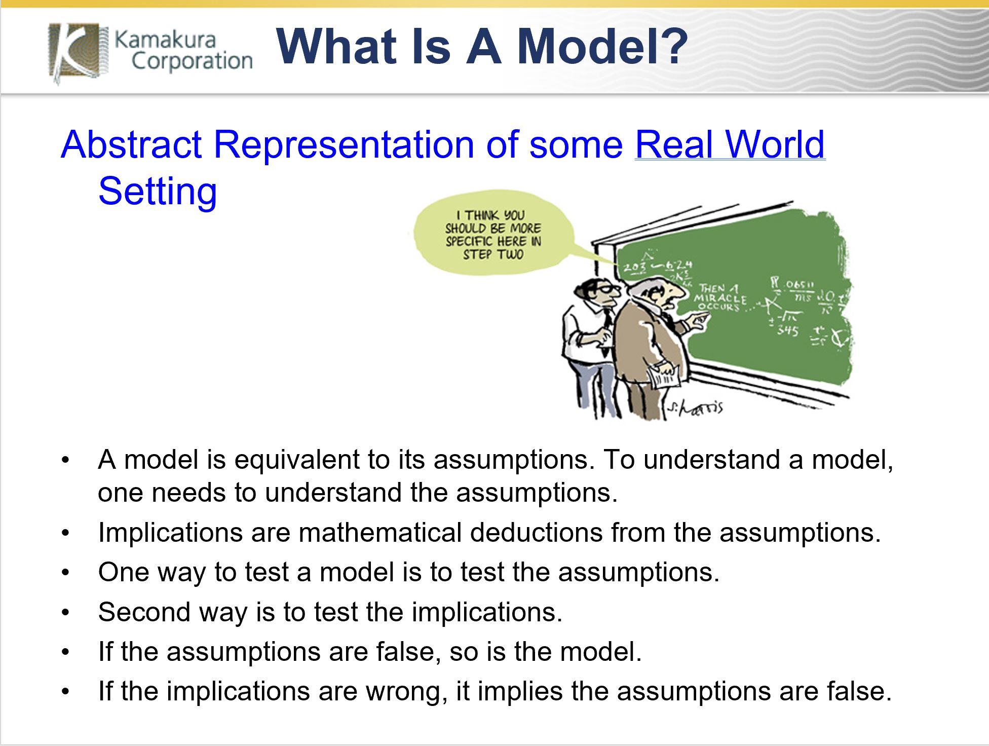
Professor Jarrow began by putting financial models in context.

A financial model is defined by its assumptions. The model’s implications are derived from those assumptions. A model can be tested both by measuring the accuracy of the assumptions and the realism of the model’s implications.
Professor Jarrow then introduced the notion of the reduced form bond model.

The reduced form bond model assumes that markets are frictionless and competitive. This assumption is relaxed in the model by the introduction of a liquidity parameter in the econometric implementation of the model.

Professor Jarrow then explained the use of a Cox process to model the default time. State variables driving this process can include both macro-economic variables and financial statement-related variables that are specific to the issuer of the risky bonds analyzed.

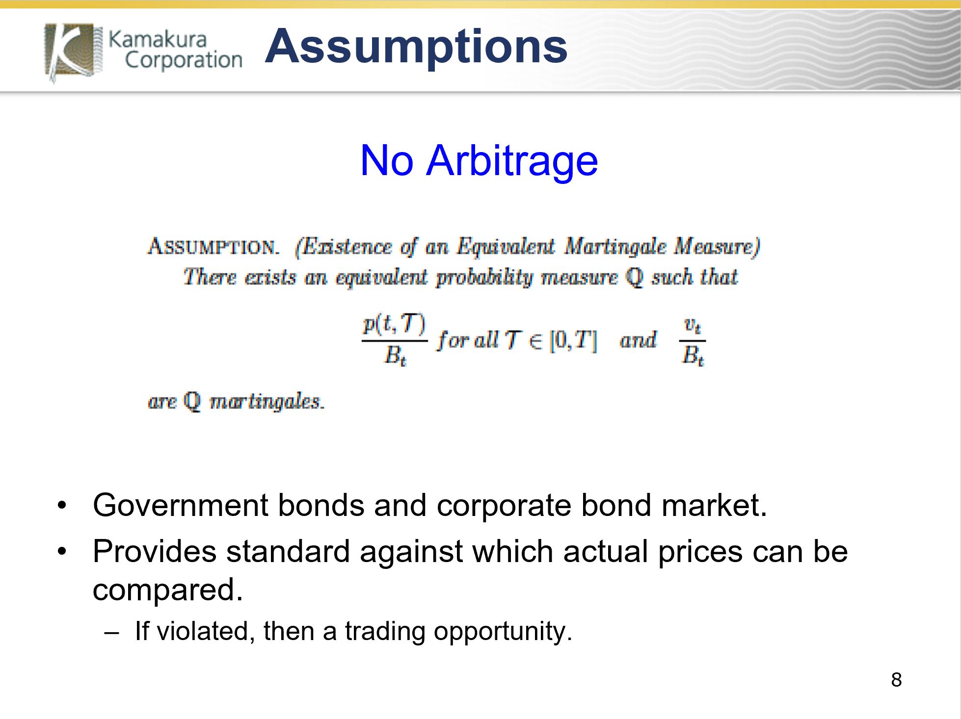
Professor Jarrow then explained the “no arbitrage” assumption invoked in the modeling process.
Professor Jarrow then described the conditional independence of risk-free interest rates, the default time, and the recovery rate under the risk-neutral probabilities in the model. This assumption is consistent with observable interest rates, default times and the recovery rate that are correlated under the observable or empirical probabilities.

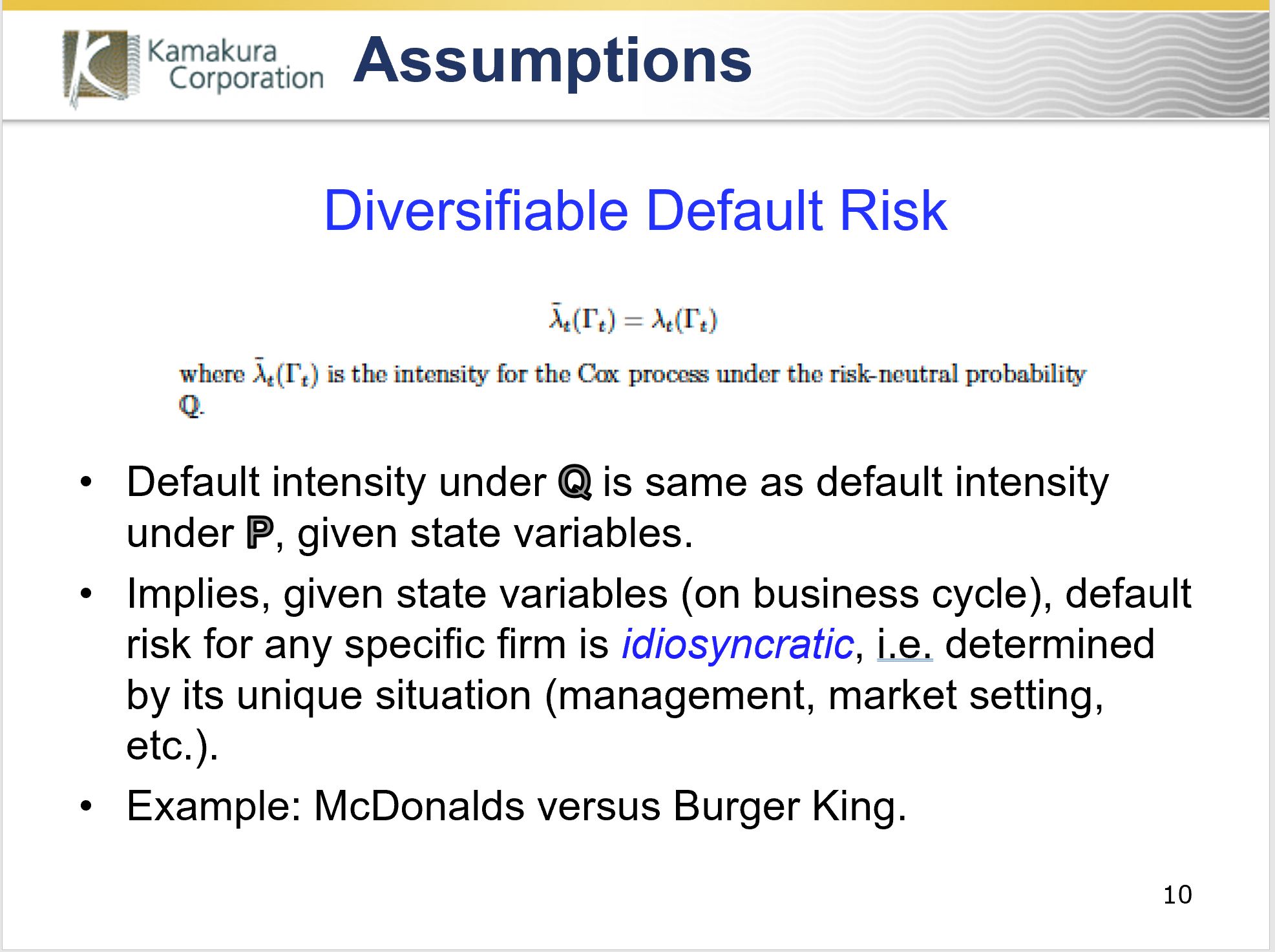
Professor Jarrow went on to explain the assumption of diversifiable default risk among firms. Conditional on the macro-economic variables, the default/no default event at a specific time is independent for any two firms.
The value of a defaultable bond can be shown to consist of digital securities that pay 0 or 1 depending on the default status of the firm.

An extension of the model includes discounts for both types of digital securities for liquidity reasons.

Professor Jarrow introduced the computational issues that Dr. van Deventer will cover in the second half of the presentation.

In closing Professor Jarrow summarized the cost of “term insurance” on the bond.

At that point Dr. van Deventer began his discussion of the theory and empirical derivation of the bond/CDS basis.

Dr. van Deventer introduced simpler notation for the coupon 0/1 securities c, the 0/1 recovery securities in each payment period r, the dollar coupon paid semi-annually K, and the recovery rate δ.

The reduced form value of a bond is the sum of the principal amount 100 times the final all or nothing coupon security, the N coupons of K dollars times the corresponding 0/1 coupon securities, and finally the sum of N 0/1 recovery securities times the principal of 100 and recovery rate δ. Note that there is no recovery on coupons, so principal is in fact SENIOR to coupons.
In the next slide, Dr. van Deventer showed the formulation of coupon securities and recovery securities. He applied the liquidity discount to coupon securities, but he assumes “no arbitrage” constraints that require the sum of the period 1 coupon security and period 1 recovery security to have a total value equal to a 1 period Treasury bill. Why? Because the holder of a 1 period coupon security and 1 period recovery security receives $1 in every scenario, default or no default. For period 2 and subsequent payment periods, the no arbitrage constraint is slightly different.
The difference between that specification and the specification applied by Professor Jarrow is a key empirical question.

In the next slide, Dr. van Deventer used the building block securities to calculate the present value of a new credit default swap that has payment periods half as long as the semi-annual bond payment periods. The dollar amount paid in advance for credit insurance is S/4 dollars per quarter. S is the annualized credit default swap spread. Note that there is no Libor/swap curve or SOFR/swap curve in this equation.

In a competitive market for a derivative for which there is zero up-front payment (other than the first credit insurance payment, which we account for separately), the market value must be zero to avoid arbitrage. This allows us to solve for the annualized credit default swap rate implied by the credit risk of the borrower, conditional on the recovery rate and liquidity parameter.

Dr. van Deventer then gave the explicit formula for the bond/CDS basis. The formula depends on the credit spread, calculated precisely, on two newly issued securities: a new issue with N semi-annual payments from the reference issuer, and a similar new issue from a risk-free (approximately) issuer like the U.S. government. We assemble the par coupon yields to get the new issue coupons of 2K* and 2Krf*. The difference between these par coupon yields is the credit spread, of course. Note that we do not use the yield to maturity of an existing bond in this calculation, because the many false assumptions embedded in the yield to maturity calculation (the biggest of which is the assumption that all payments will be made with certainty) introduces noise to the bond/CDS basis.

At this point Dr. van Deventer introduced the default probabilities and traded credit spreads from Kamakura Risk Information Services (KRIS). For more information on KRIS reduced form default probabilities please use this link:
https://www.kamakuraco.com/solutions/kamakura-risk-information-svcs/default-probability-models/
For this presentation, the reference name used in the example is Ford Motor Credit Company LLC. It is assumed as a first approximation that the default probabilities of FMCC are identical to those of Ford Motor Company, which are taken from KRIS on each business day.

Next, Dr. van Deventer explained that traded credit swap prices are still undisclosed to the public despite the fact that those prices are known to the Depository Trust and Clearing Corporation. Accordingly, using CDS quotes is the only option for this analysis, but first it needs to be confirmed that CDS are regularly traded on the Ford corporate family. The next slide from KRIS confirms that there is steady weekly volume so the CDS quotes should have some basis in reality.

Dr. van Deventer then explained Step 1 in the analysis: the generation of the maximum smoothness forward rate curve for the U.S. Treasury on every trading day. This was done using Kamakura Risk Manager version 10. More information on KRM is available here:
https://www.kamakuraco.com/solutions/kamakura-risk-manager/

Dr. van Deventer then explained the two-step process that Kamakura uses to calculate the bond-implied recovery rate and liquidity parameter for each issuer.
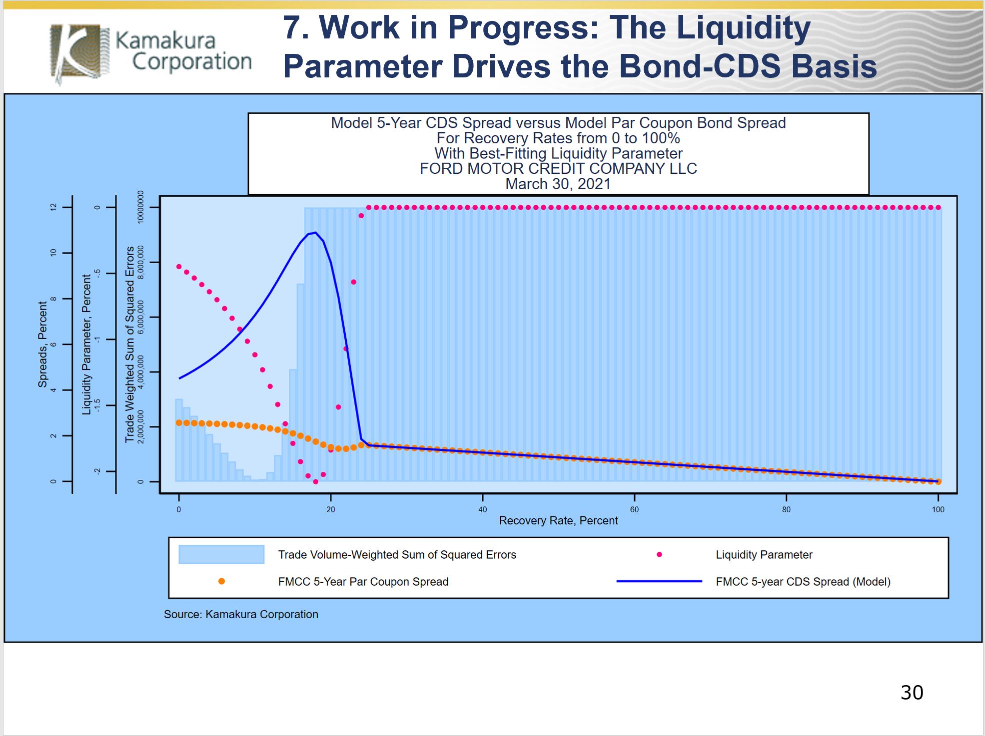
The first of the two steps calculates the liquidity parameter that minimizes the sum of squared bond pricing errors for the assumed recovery rate value. 101 recovery rate values are used in this analysis, from 0% to 100% in 1% increments. This analysis shows that the approximate solution is a recovery rate of 10% and a liquidity parameter of minus 0.1116 (minus 1.116%).

Dr. van Deventer then showed how the final values for these two parameters are derived from a powerful non-linear equation optimizer using the starting values shown in the slide above:

The best-fitting parameter values were 10.427% for the recovery rate and minus 1.163% for the liquidity parameter. These parameters are fitted for every business day in the example.
Using the smoothed U.S. Treasury curve, the 5-year par coupon Treasury yields are calculated on every business day. Using the smoothed U.S. Treasury curve and the daily values for the recovery rate and liquidity parameter, the 5-year par coupon yield for a new Ford Motor Credit bond issue is calculated. The difference is the true credit spread (not the market convention using yields to maturity).
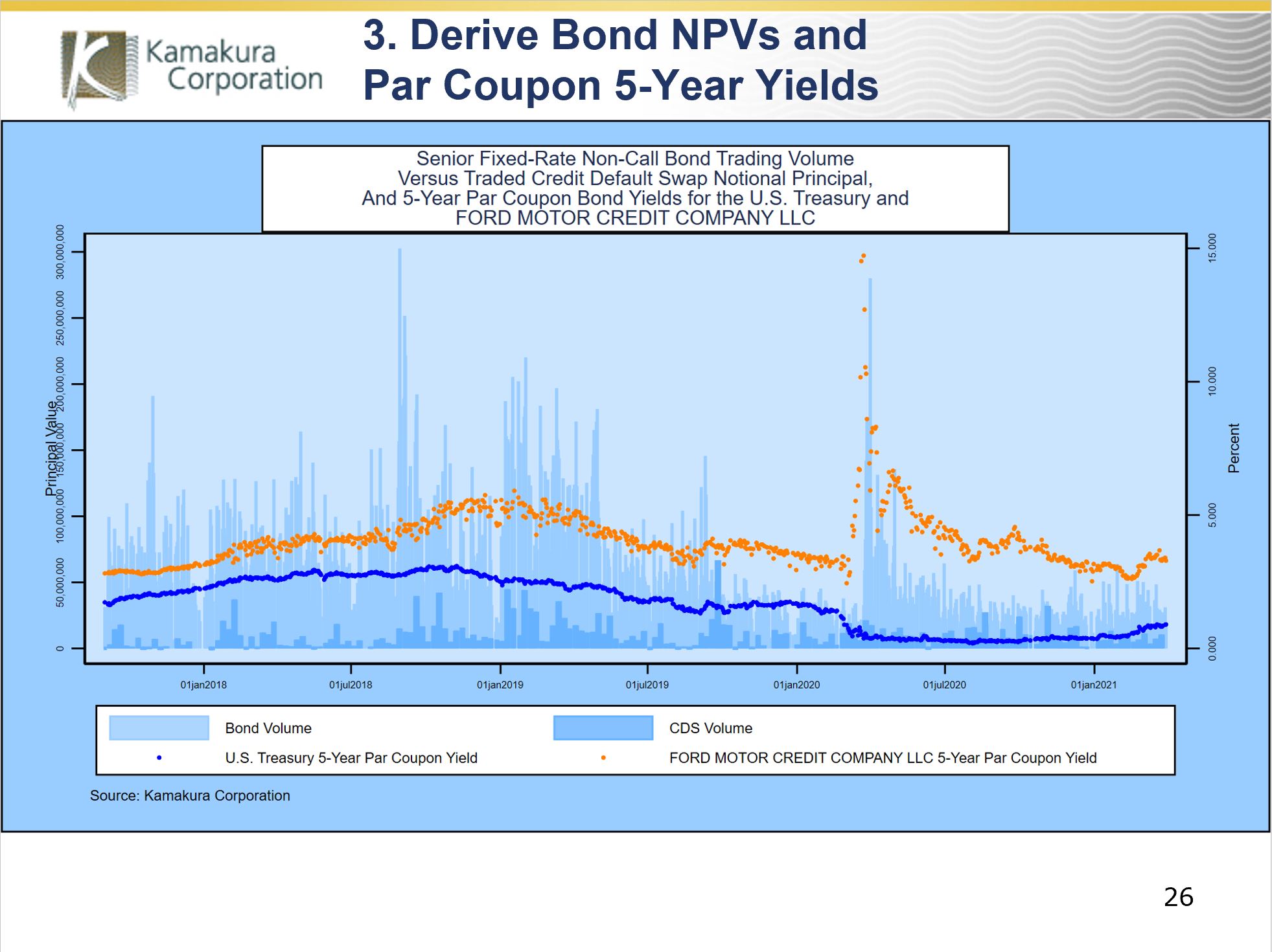
This credit spread is plotted in orange in the next slide. The blue dots represent the no arbitrage credit default swap spread that comes from the reduced form building block derivation given above. For most of the time series studied, the credit spread and CDS spread are nearly identical, differing only because of differences in timing (such as pay in advance on the CDS) and frequency (quarterly versus semi-annual). This held even for the sharp spike in credit spreads with the onset of the covid-related bond market panic in March and April 2020. What happened on the right-hand side of the graph, when the theoretical credit default swap spread deviated significantly from the credit spread?

The next slide is helpful in understanding what is going on. The green dots added to the graph represent the CDS quotes for the Ford family. Note that at the peak of the virus crisis, the CDS quotes were generally higher than both the model-implied credit spread (orange) and CDS spread (blue). On the far right-hand side of the graph, the CDS quotes in green again converge to the model-implied credit spreads.

Why, then, is the model-implied CDS spread still high? The next slide provides some answers. Starting in September, 2017, we plot daily values for the liquidity parameter (in orange) versus the recovery rate implied from bond prices for Ford Motor Credit. For the same sections of the graph, the moving average of the liquidity parameter is very close to zero and the recovery rate fluctuated in a reasonable range. On the far right hand side of the graph, Ford Motor Credit bond prices changed in such a way that the implied recovery rate fell to zero and the liquidity parameter became a more negative number.

The next slide analyzes the interaction of the liquidity parameter and recovery rate on March 30, 2021, the same date we used to derive the recovery rate and liquidity parameter above. As we did above, we vary the recovery rate in 1% increments from 0% to 100%. For each level of recovery rate, we derive the liquidity parameter that minimizes the sum of squared errors. We overlay the par coupon credit spread (orange) and swap spread implied by the parameters for every level of recovery rate and the corresponding liquidity parameter. The graph shows that once the “best fitting” liquidity parameter goes to zero, the model-implied credit spread and model-implied CDS spread converge.
The specification used for how the liquidity parameter affects coupon securities and recovery securities is clearly the key to the CDS/bond basis.
For those readers interested in Kamakura’s conclusions in this regard, please contact Kamakura for more information at info@kamakuraco.com.