Interest Rate Hedging when Using a Multi-Factor Heath, Jarrow, and Morton Model: United Kingdom, September 4, 2026

Interest Rate Hedging when Using a Multi-Factor Heath, Jarrow, and Morton Model: United Kingdom, September 4, 2026

• Donald R. van Deventer
• First version: June 18, 2025
• This version: September 4, 2026

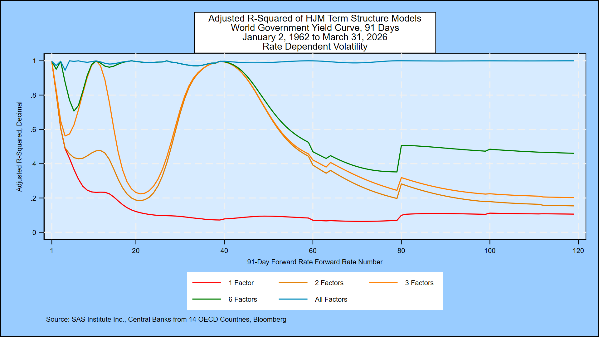
For almost 90 years, the hedging of a fixed income portfolio or a financial institution’s balance sheet has been focused on duration and its derivative, convexity. Duration assumes that the yield curve is flat, that the time intervals between payments are identical, and that yield curves for two bonds of the same issuer can have different flat levels. Duration hedging implicitly assumes that only one factor is driving yield curve movements. With the introduction of the Heath, Jarrow and Morton [1992] no-arbitrage multifactor interest rate modeling framework, there have been enormous improvements in interest rate analytics. Fitting of multifactor models to yield curve histories are much more accurate, and forward-looking simulations using “HJM” can price the relevant bond prices perfectly, not only at time zero but also for a holding period of any length. The graphic below compares the in-sample quality of fit for a 14-country “World” government yield database. The 12-factor “all factor” adjusted R-squared (in blue) is close to 100%, while the 1-factor model (in red) is below 20% after the first few quarterly yield curve segments:

With this background in hand, we introduce a brief discussion of hedging in a multi-factor HJM model.

Three Approaches to Hedging

Common practice in many financial institutions, like the failed Silicon Valley Bank, often focuses on near-term net income. Best practice financial economics, however, is always focused on market values and a mark-to-market approach. We use that approach in this note.

Hedges can be done both at the transaction level and the portfolio level for any number of hedging instruments. The “best hedge” is that which minimizes the variation in the value of the underlying assets less the value of the N hedging instruments

• CONTINUOUS TIME “DELTA HEDGE” using derivative of value change with respect to the M underlying risk factors at time 0
• DISCRETE TIME HEDGE using Ito’s lemma to outline value changes with respect to the M underlying risk factors at time 0
• NUMERICAL OPTIMIZATION that minimizes the variation in the hedge value by selecting the best weights on the N hedging instruments, taking all M risk factors into account at time 0 using full forward simulation

In general, the most accurate hedge for a specific holding period can be derived using calculus, Ito’s lemma, or simulation. The first two methods use the derivatives and formulas in Jarrow and van Deventer [2020]. For purposes of this note, we take advantage of a simulation to derive a ranking of alternative hedging strategies using linear regression.

In this worked example, we use the results of a 12-factor Heath, Jarrow and Morton simulation of the United Kingdom Gilt yield curve 30 years forward using 91-day time steps. For expositional purposes, we assume that the underling portfolio has the cash flows of a 10-year Gilt with principal of £100.00 and which pays semi-annual coupons (we are using semi-annual coupons for expository purposes) at a 5% rate, £2.50 at the end of each even-numbered 91-day period. Using both the spot Gilt yield curve on September 4, 2026 and the simulation, this underlying portfolio has a known market value. We assume without loss of generality that the universe of hedging instruments includes zero-coupon bonds maturing at the end of each 91-day period out to 40 periods and par coupon bonds at the normal “on-the-run” maturities.

A perfect hedge exactly replicates the cash flows of the underlying portfolio. In this case, the perfect hedge is obvious: we short zero-coupon bonds with maturities of 2, 4, 6,…40 periods with a principal amount of 2.50. We also add £100 principal of zero-coupon bonds with a maturity of 40 periods. A simulation-based optimization shows the perfect hedge, as it should, has a standard error of zero and an adjusted R² of 1.0000 for this regression:

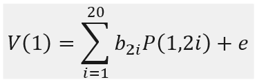
The left-hand side is the value of the portfolio at time step 1, the first time step with 50,000 Monte Carlo simulation results. The hedging instruments are the 20 zero-coupon bond prices at time step 1 with initial maturities of 2, 4, 6,…40 periods. The second chart below confirms that this hedging portfolio perfectly replicates the underlying portfolio’s cash flows and therefore has a root mean squared hedging error of zero.

We now want to answer this question: how does the hedging accuracy change when we use a different set of hedging instruments? We start by asking “What is the most accurate single instrument zero-coupon hedge?” The answer, using root mean squared error as our measure of accuracy, is given in this chart:

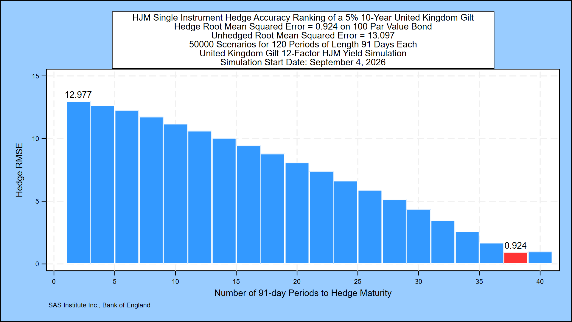
The most accurate single instrument hedge is to sell short a zero-coupon bond with a maturity of 38 periods. The root mean squared error is 0.924, substantially less than the unhedged RMSE of 13.097. Although many risk analysts are still using term structure models with the shortest maturity as the “risk factor,” a hedge using the two-period zero-coupon bond as a hedge is nearly useless. Its root mean squared error, at 12.977, is only slightly better than an unhedged position.

Next we pose an obvious question: how does hedge accuracy change if we add a second instrument to the hedge? The answer is shown below:

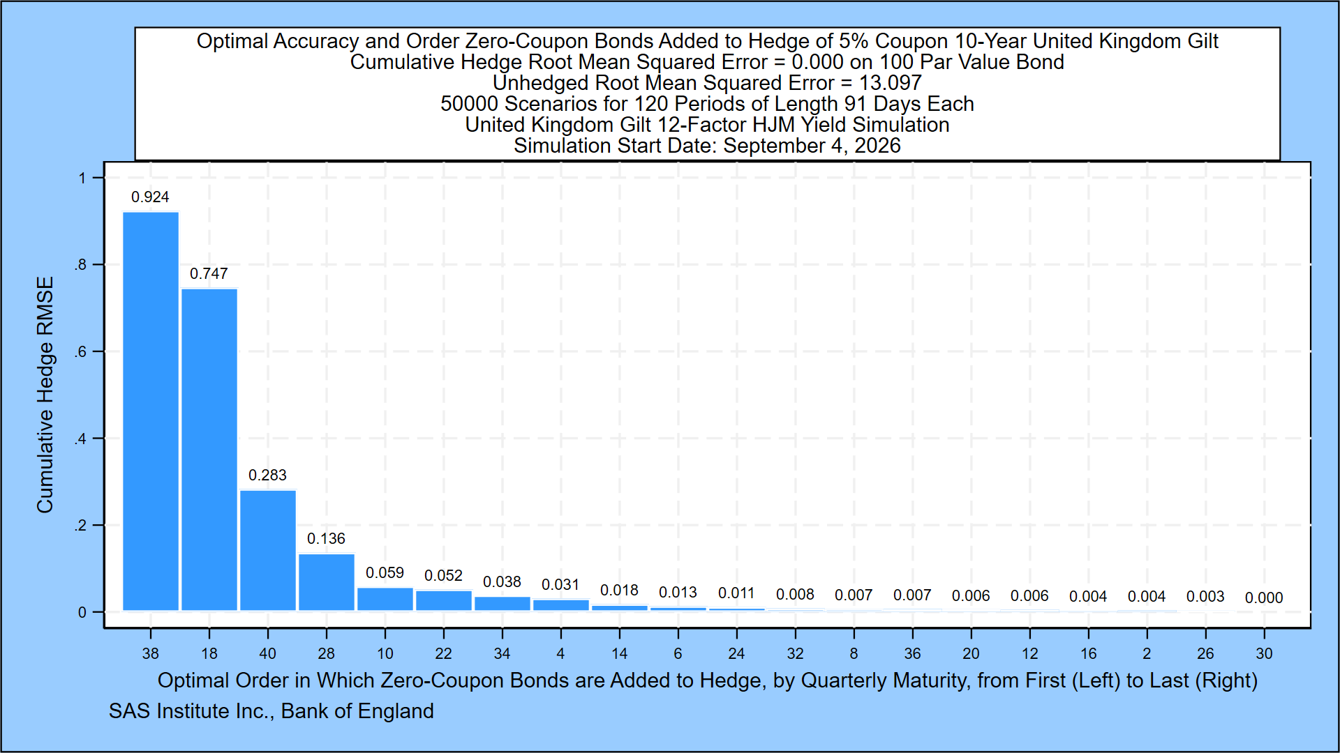
The chart shows the root mean squared error drops from 0.924 to 0.747 if we add an 18-period zero-coupon bond to the hedge (as indicated by the x-axis labels). If we add a third instrument, the best instrument to add is the 40-period zero-coupon bond to the hedge. That reduces the root mean squared error to 0.283 for a £100 par value bond. Additional instruments can be added from left to right, reducing hedging error to zero when the 20 hedging instruments described above are used to perfectly match cash flows of the underlying “portfolio.”

We can also consider using par coupon bonds as a hedging instrument. The hedging accuracy using portfolios of par coupon bonds is shown in this graphic:

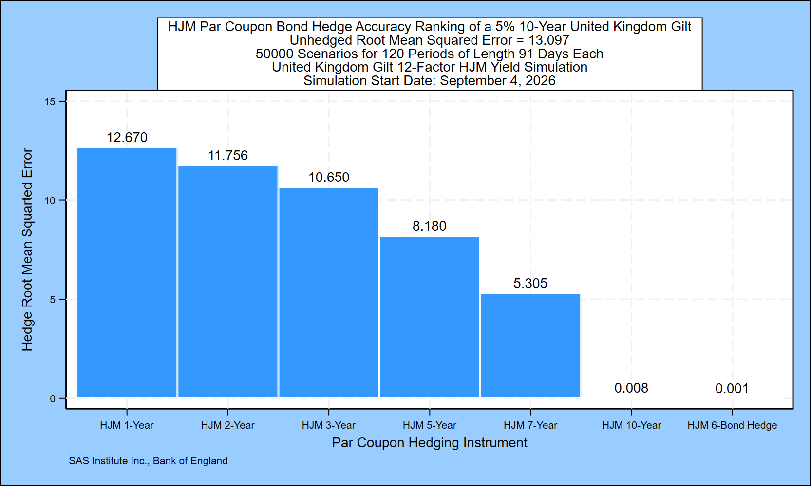
Note that the hedging error of a 10-year par coupon bond has a root mean squared error of 0.008, while a portfolio of six par coupon bonds reduces the hedging error still further to 0.001.

Finally, we can consider the best hedge using any portfolio of par coupon bonds and zero-coupon bonds.  We find that, in addition to the 20 zero-coupon bond portfolio analyzed above, one 10-year par coupon bond and the 10-year zero-coupon bond in combination also form a perfect hedge:

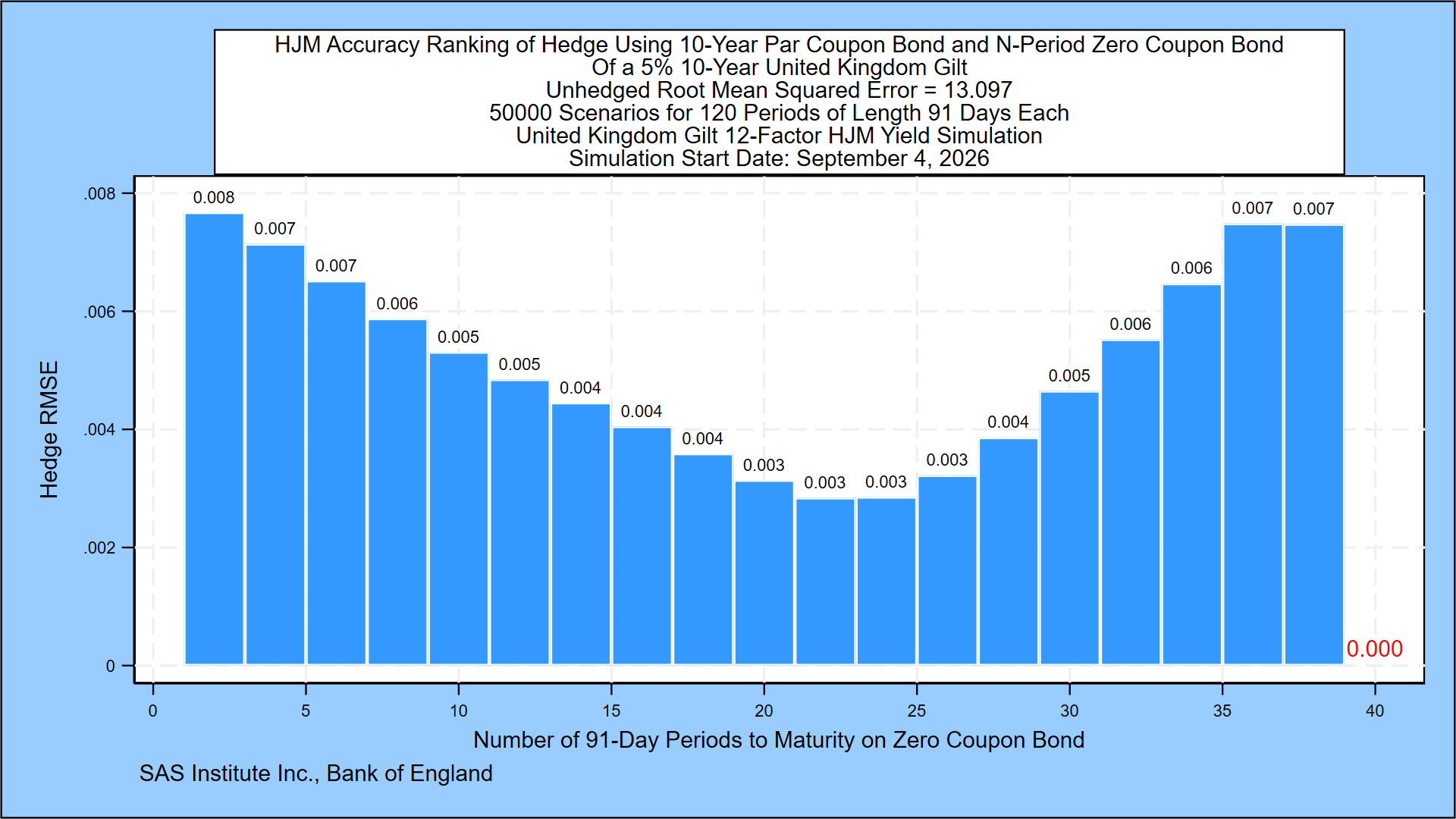
It is straightforward to run regressions for any combination of the hedging instruments and for any number of hedging instruments in an automated way, as we have done in this example.

Pseudo Code for Hedge Effectiveness and Optimization Using Zero-Coupon Bonds

1. Run a significant HJM simulation for the government yield curve of interest.
2. Enumerate the complete list of hedging instruments for each possible number of hedging instruments, in this case from 1 through 20. That gives a number of hedges to test, say N.
3. Run a linear regression for each possible single instrument hedging strategy from 1 to N
4. Rank them from best to worst.
5. Add the best instrument (the 38-period zero-coupon bond) to the ideal hedging portfolio.
6. To determine the best addition to the hedge, we run a linear regression that predicts the underlying portfolio’s value as a function of both the best single instrument maturity (38-periods) and each of the remaining zero-coupon bond maturities. We add the best additional maturity (22 periods) to the ideal hedging portfolio.
7. We repeat this process to determine the best hedging portfolio with 3 instruments, 4 instruments and so on until we match the known result for the 20-instrument ideal hedging portfolio.

An alternative approach is to use stepwise regression to add explanatory variables to the hedging portfolio as long as each incremental instrument produces a statistically significant improvement in accuracy. The author’s experience so far shows that this approach, while logical, sometimes falls short of the answer that financial theory shows is the perfect hedge.

References

Jarrow, Robert A. and Donald R. van Deventer, “Monte Carlo Simulation in a Multi-Factor Heath, Jarrow and Morton Term Structure Model, Technical Guide” version 5.0, SAS Institute Inc. memorandum, August 27, 2020.