Robert A. Jarrow[1] and Donald R. van Deventer[2]
Presentation to Risk Americas, May 11, 2022
This Version: May 19, 2022
Abstract
We present an annotated version of slides used in a presentation to Risk Americas on the reduced form approach to SOFR swap and swaptions valuation. The same methodology can be used for any floating rate swap index from Libor to Treasury bills and to any new short-term index that may emerge in the years ahead. The contents of the slides were co-authored by Prof. Jarrow and Mr. van Deventer. The annotated comments which follow reflect comments from the podium by Mr. van Deventer or additional remarks that reflect the newer data used in this version and comments from conference participants received after the original presentation.
From an academic point of view, Prof. Jarrow often comments that a model based on false assumptions should be rejected. From a practitioner point of view, a model based on false assumptions cannot be rejected until a more accurate replacement model is available. This presentation is candid in its assessment of models in common use for swaptions valuation and practical in replacing false assumptions with alternatives that fit observable market prices perfectly.
Comments and suggestions are welcome at info@kamakuraco.com.
A PDF version of this note is available here:
Kamakura-ReducedFormValuationSOFRSwaptions20220511
This version of the presentation uses data as of May 13, 2022 instead of the April 22 data discussed on May 11.
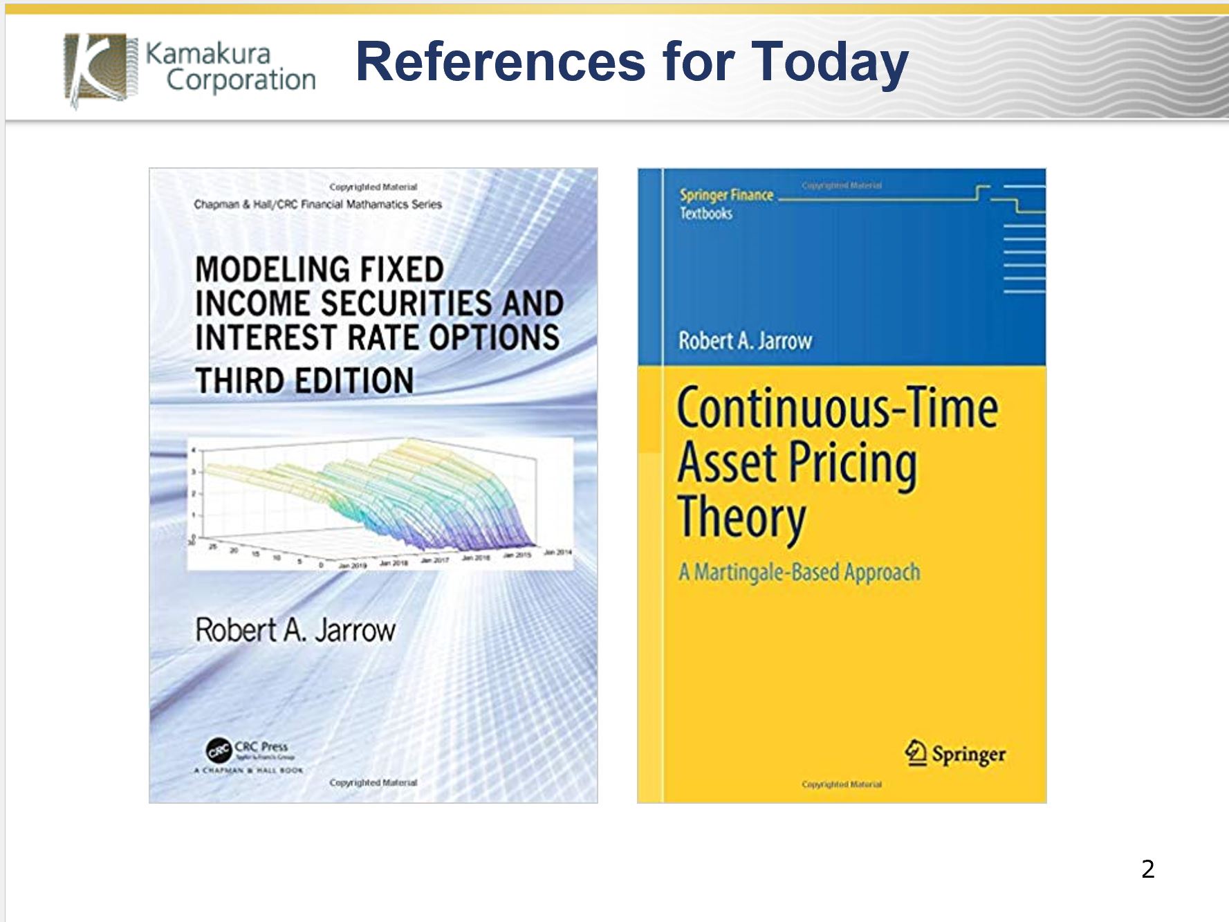
The methodology discussed today is not new. It was developed in the late 1980s by Prof. Jarrow, Andrew Morton, and David Heath. The academic version of the paper was published in 1992 in Econometrica, the “HJM” approach to term structure modeling. That approach derives the conditions for no arbitrage (i.e., a perfect fit to market data) for any number of factors and any form of factor volatility. Because there can be many factors, the word “volatility” by itself has no meaning, unlike current market convention for swaptions valuation. These recent works provide extensive worked examples (on the left) and a consistent mathematical framework (on the right) for what follows.

Because Prof. Jarrow was unable to be present at the conference, Mr. van Deventer was speaking without his favorite “mathematical bodyguard.” For that reason, the only math in this presentation consists of addition, subtraction, multiplication and division.

Two irresistible forces collide when it comes to the valuation of swaps and swaptions. The first group is passionately devoted to Excel spreadsheets and two probability distributions: the normal and lognormal distributions. The second group is the uneasy collaboration between regulators, who have grown weary of corruption by dealers, and the dealers themselves. SOFR was forced on market participants as the one interest rate that is most difficult to manipulate. The authors belong to neither of these groups, although Mr. van Deventer was a long-time card-carrying member of the Excel/normal group. He has since moved on to more powerful tools.

From an academic point of view, it is easy to argue that SOFR is the equivalent of a 1-day Treasury rate, but this quote from the Financial Times makes it clear that SOFR is much more than that.

This exchange, after the presentation, explains why SOFR is NOT equivalent to a 1-day Treasury. A repo trader made it clear that there is definitely a credit component embedded in the repo rates from which SOFR is derived by the Federal Reserve Bank of New York. The data which follows confirms this view quite clearly.

In what follows, we use best practice financial economics and the generalization of the Black-Scholes risk-neutral valuation to eliminate a series of false assumptions commonly used to value swaps and swaptions. We highlight those differences in the slides that follow.

On this slide we plot U.S. Treasury par coupon yields, U.S. Treasury zero coupon yields, U.S. Treasury monthly forward rates, and SOFR swap quotes out to 30 years as reported by Bloomberg. SOFR swap rates, in part due to differences in day count basis, differ significantly from par coupon Treasury yields. We explain why in the following slides.

Most of the worry about SOFR as an index is the ex-post compounded floating rate payment. In this table we use daily Treasury yields since January 1962, smoothed to provide discount factors from 1 day to 30 years for every observation date. Using overlapping time intervals from 7 days to 18 months.[3] We run a regression of this form:
Compounded SOFR = alpha + beta (time 0 fixed dollar interest on matched maturity fixed rate Treasuries)
Note the “beta” in this equation declines with maturity and that the alpha is usually small.

This graph shows the dispersion (we try to avoid the term “volatility”) of compounded SOFR or 1-day Treasury (depending on SOFR availability) around the fixed dollars of interest on U.S. Treasuries over the full time period.

One of the reasons for the decline in beta on a data set that is mainly 1-day Treasury yields is the term premium embedded in U.S. Treasuries. This graph, updated weekly on www.kamakuraco.com, shows the difference between the time zero U.S. Treasury zero coupon bond yield curve versus the total return on the compounded return on expected empirical (not risk-neutral) 3-month Treasury bill yields in a 10-factor Heath, Jarrow and Morton simulation of 500,000 scenarios that we explain in later slides. We need to determine whether this is relevant to SOFR swaps and swaptions.

Now we turn to SOFR swaps first and derive what alpha and beta values are implied by observable SOFR swap yields.

To do this, we use the extremely powerful approach of Amin and Jarrow (1992), which shows how to do valuation of any non-defaultable instrument in an environment where the risk-free curve is driven by multiple factors and volatility that can be either random (driven by rate levels, for example) or simply time dependent. We assume the swap and swaption counterparties are risk-free as Black and Scholes did. We note that an individual repo counterparty can default, but the SOFR index does not. For that reason, Amin and Jarrow’s approach is appropriate.

This slide summarizes the differences between best practice financial economics and common practice for swap and swaptions valuation. The most important difference is that all discounting is based on the risk-free yield curve. Specifically, a forward-looking simulation is used to generate the daily compounded value of a Treasury “money market fund” that takes on a different value in each scenario at each time step. Proper procedure does not use a constant discount rate (Black-Scholes did so only because they assumed rates were constant). Moreover, the relevant yield curve for discounting is NOT the swap “curve” (which is not a yield curve). In this analysis, we derive the swap curve, rather than using it as an input to valuation.

This slide summarizes how the Heath, Jarrow and Morton approach provides a Monte Carlo simulation that perfectly values not only the time-zero U.S. Treasury curve but also perfectly prices future returns for any maturity and any holding period. Using 120 quarterly yield segments of the May 13, 2022 U.S. Treasury curve, the Monte Carlo simulation is generated such that the risk-neutral expected value of the 120 zero coupon bond prices matches their value exactly. We use this knowledge to derive valuations that apply to all simulations, not just the simulation we performed on May 13.

Using the Amin and Jarrow approach, we know the value of the first fixed dollar payment on a SOFR swap for S dollars in N days is the risk-neutral value of S discounted by the U.S. Treasury daily money fund value in each scenario. Because S is not correlated with future interest rates, it comes outside of the expectation. The value is simply S times the zero-coupon Treasury bond that matures on the date S is paid. The use of the “swap curve” to extract a discount factor is simply as wrong as it is common.

The value of the fixed payments (m in total) on a SOFR swap is just S dollars times the m zero coupon U.S. Treasury zero coupon bonds maturing on the m payment dates. The only information we use from the swap market is the dollar amount of the fixed payment. Note that the value of all fixed payments does not equal the notional value of the swap.
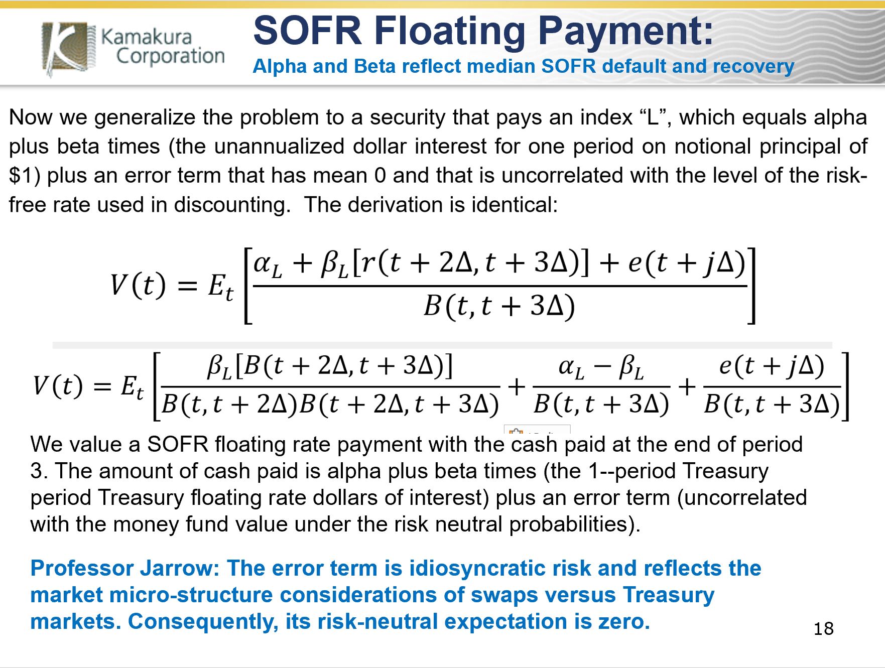
Now we use the same approach to value one floating leg of the swap, taking the third floating rate payment as an example. We know from previous slides that repos have a non-zero default risk and a recovery rate that is not necessarily 100% in the event of default. As a first approximation for this risk above and beyond the one-day Treasury, we assume the compounded SOFR rate paid at the end of period 3 is alpha plus beta times the dollars of interest r that would be paid on a compounded 1-day Treasury rate, plus an error term. When we recognize that we have a Treasury money market fund component in both the numerator and the denominator and take risk-neutral expectations, magic happens.

Without doing any simulations, risk-neutral valuation gives us an explicit formula for the 3rd floating rate payment that is a function only of alpha, beta, and the U.S. Treasury zero coupon bonds that mature at the end of periods 2 and 3.
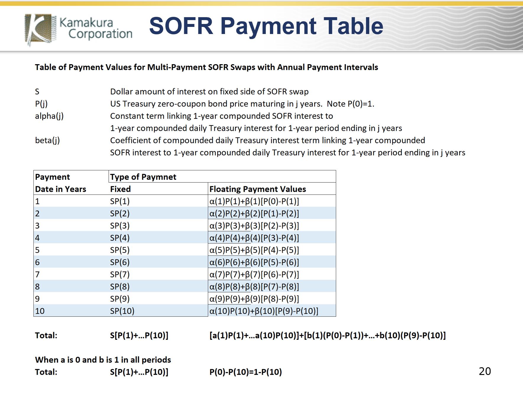
This table summarizes the values of the fixed and floating rate payments on SOFR swaps with annual payment dates out to 10 years. IMPORTANT NOTE: When alpha and beta are 0 and 1 respectively (as they would be if we were talking about compounded 1-day Treasuries instead of SOFR), the sum of the floating payment values is simply $1 minus the value of a Treasury zero coupon bond that matures on the last swap payment date (this happens because there is no principal exchange on the swap, contrary to common market assumptions).

For notional convenience, we let K be the sum of the Treasury zero coupon bond prices on each payment date. Vf is the value of the fixed side of the swap.

Ve is the value of the floating side of the swap. The mathematical summary here says the same thing as the table in slide 20.

Using these formulas with no simulation, we can solve for the equilibrium no arbitrage fixed dollar payments on a SOFR swap as a function of alpha and beta in each payment period (we don’t assume that they are constant) and the U.S. Treasury curve.

We can use the observable market prices on SOFR swaps and the related fixed dollar payments Sm to imply beta if alpha is assumed to be the 0.042% historical value from 1962 through April 30, 2022. That leaves us with one unknown (beta) in each period. We solve for the beta that correctly prices a 1-year SOFR swap. We then recursively repeat the process, stepping forward one year at a time, until we have beta for the first 10 years of swap pricing.

We do that for May 13 and find that the implied beta values through 18 months are consistently higher than the historical betas for the merged 1-day Treasury and SOFR data base.[4] This is consistent with the repo trader’s description of the credit risk embedded in repo quotations underlying SOFR.

Beyond 10 years, ISDA reports little trading volume. Nonetheless, implied betas can be calculated in many ways, typically using step-wise constant or smoothing generated betas. This chart shows that, if market quotations beyond 10 years have credibility, market-implied betas move up and down in fairly smooth waves.

With a perfect fit to observable swap prices in hand, we now turn to the valuation of SOFR swaptions.
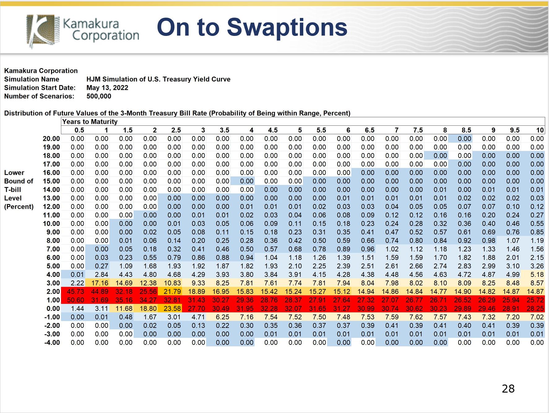
In what follows, we use a 10-factor Heath, Jarrow and Morton simulation of the U.S. Treasury curve starting on May 13 to value swaptions. An explanation and downloadable data are available here:
The simulations are updated weekly and available on www.kamakuraco.com.
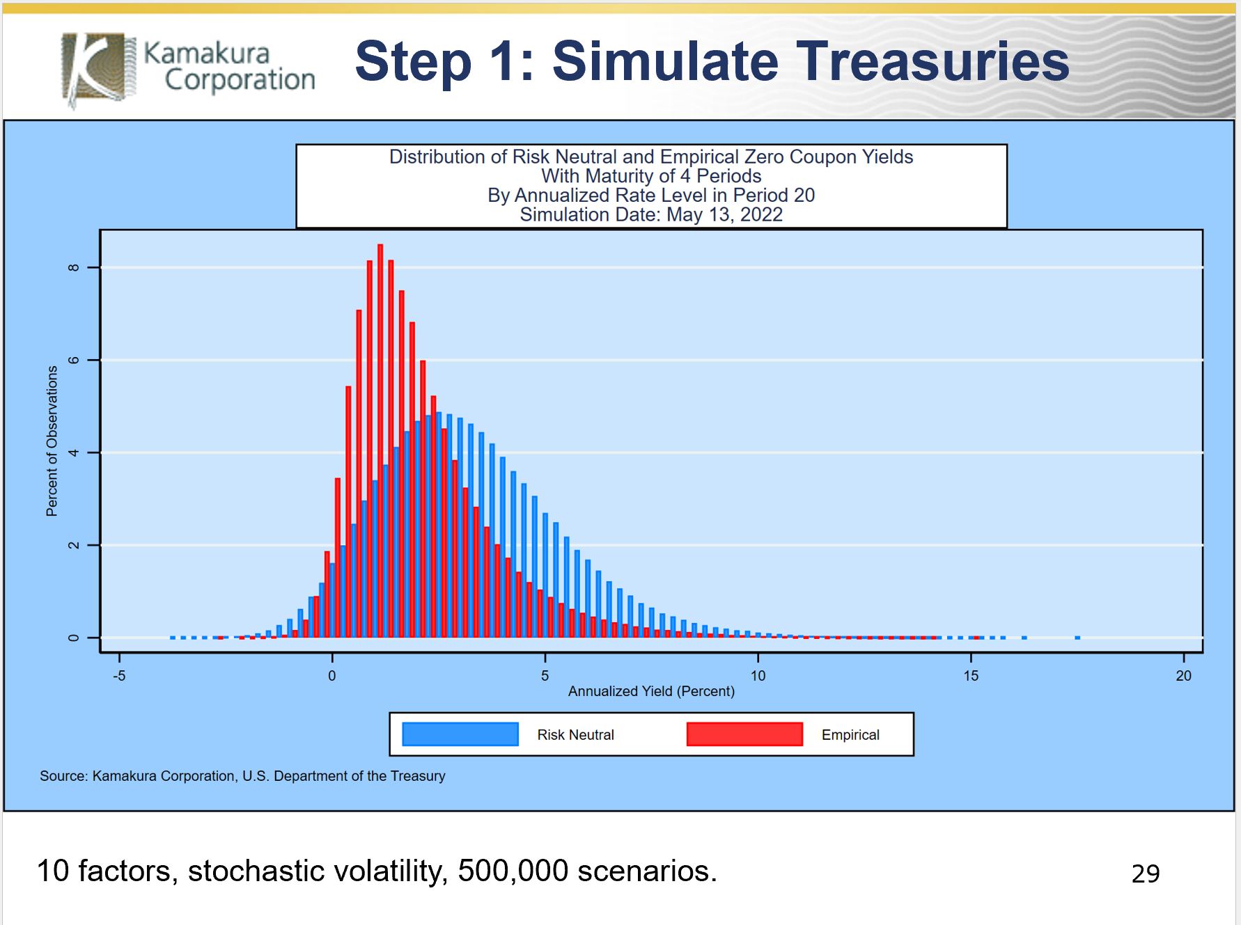
This graph shows the distinction between the risk-neutral (in blue) 1-year Treasury yield five years forward and the empirical (in red) or observable 1-year Treasury expected to prevail at that time. The difference is relevant to Black-Scholes as well: the “simulated” stock returns in Black-Scholes are the risk-neutral returns, not the actual return distribution that would be observable if one could repeat history N times.
The use of 10 factors is essential to replicating the actual level of volatility that has appeared across the U.S. Treasury curve throughout the 60-year history in the data set. If an analyst fit a model to history using only one factor, a separate Kamakura study shows that the simulated dispersion of interest rates would underestimate actual dispersion by 61% to 83%.

Using these simulations, we now have two equations in 2 unknowns at each annual time step from 2 years[5] onward: we have the 2-year SOFR swap rate and the quote for a European swaption with an exercise period of 1 year on a swap with an underlying maturity of 1 year on the exercise date. We fit alpha and beta so that both the swap and the swaption are priced perfectly. Ultimately, we do not constrain alpha to be non-negative.

With only a small incremental calculation, we calculate the forward levels of the fixed dollar payment on the underlying 1-year forward swap using the existing Treasury simulation and any equation solver (including Excel) such that the swaption and the 2-year SOFR swap are priced with no error.

If we assume physical delivery of the underlying swap, the positive cash flows on the underlying swap versus the strike dollar payments will come at the end of year 2, so discounting is done using the 500,000 values of the U.S. Treasury money market fund in year 2. The value of the swaption is the average of the discounted values (roughly half of which will be zero since it will not be rational to exercise the swaption).

This approach can be used on the full matrix of swaption prices, but the authors prefer to use only those maturities for which there is a high confidence that quoted dollar swaption prices are consistent with real traded prices, not a back-office broker model alone.

This graph shows the distribution of the simulated 1-year SOFR swap rate 4 years forward using the best fitting alphas and betas for years 1 through 5. Exercise is rational when the graph is shaded yellow. Profits are zero when exercise is irrational, shaded blue. The distribution is not normal (the black line) for a number of reasons:
- The Treasury simulation uses 10 factors, not 1
- The Treasury factor volatilities are stochastic, driven by rate levels, not normal
- The evolution of alpha and beta may in fact be random
The skewness and kurtosis are given in the notes to the slide.

Black and Scholes assumed interest rates were constant, which is why they appropriately used a constant discount rate for all stock price scenarios. When valuing interest rate derivatives that only exist because interest rates are random, it is simply wrong to use a constant discount rate instead of the scenario-specific money fund values. This example shows that the use of a constant discount rate to value a European swaption can result in very serious mispricing. For a 9-year exercise period on a 1-year underlying swap, the true value of the swaption is 169 basis points, but a model with 1 discount rate at the time zero 10-year US Treasury zero coupon bond yield wildly overestimates swaption value at 197 basis points. The reduced form model prices the swaption (and the underlying term structure of swap prices) perfectly.

In the next slide we compare the perfectly matched observable market prices for European swaptions on a 1-year underlying SOFR swap with a hypothetical swaption: using the same strike price, we set the alphas to zero and betas to one to price a swaption where the floating rate index is the compounded 1-day Treasury yield, not SOFR.
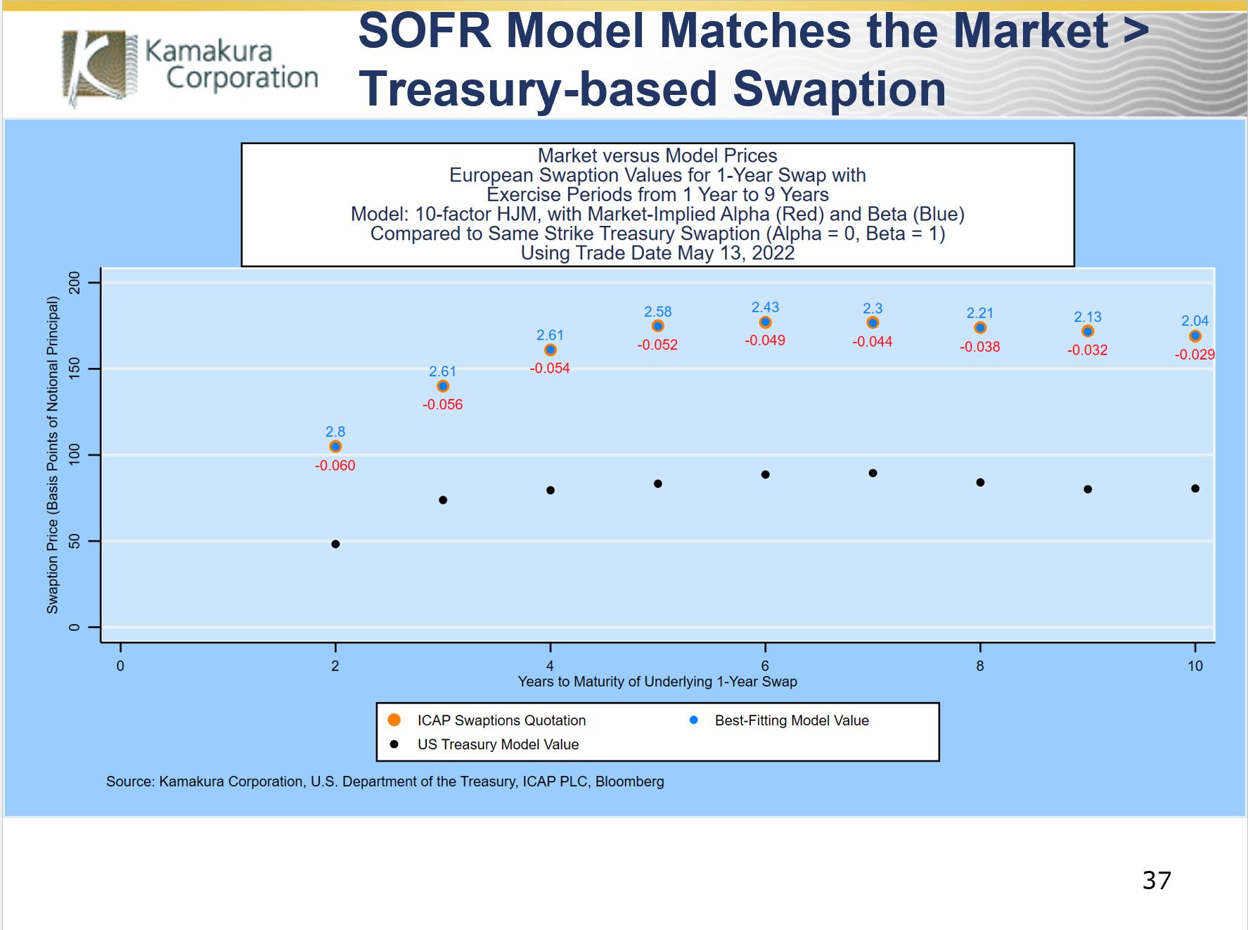
The cost of the SOFR swaption is usually more than double the price of a swaption using the compounded 1-day Treasury rate. When it comes to hedging interest rate risk, a SOFR swaption has alpha and beta “parameter risk” in addition to risks stemming from movements in the underlying Treasury curve.

We conclude that a reduced form model for SOFR swaps and swaptions valuation is essential to the transparent understanding of fair value, hedge ratios, and interest rate risk. We welcome comments, questions, and suggestions at info@kamakuraco.com.
Footnotes
[1] Samuel Curtis Johnson Graduate School of Management, Cornell University, Ithaca, N.Y. 14853 and Kamakura Corporation, Honolulu, Hawaii 96815. Email: raj15@cornell.edu
[2] Kamakura Corporation, Honolulu, Hawaii 96815. Email dvandeventer@kamakuraco.com
[3] We apologize that the adjusted r-squared for 546 days is not correct due to inevitable Excel errors.
[4] SOFR data was not reported by the Federal Reserve Bank of New York until April, 2018.
[5] For the first-year alpha and beta, we use the historical alpha and the implied beta derived using the 1-year SOFR swap quote alone.


