Model Validation: Proof that 1-factor Interest Rate Models
Underestimate Risk by 61% to 83%
Donald R. van Deventer[1]
First version: March 17, 2020
This version: March 23, 2021
Abstract
We use daily observations of the U.S. Treasury yield curve from 1962 to 2020 to construct two state of the art Heath, Jarrow and Morton term structure models. Both models incorporate stochastic interest rate-driven volatilities, generate both empirical and risk neutral interest rates, allow negative rates, and recognize that interest rate volatility is positive, not zero, when forward rates are zero or negative. The models were both derived in the same manner using a widely available statistical package from StataCorp LLC. Both models correctly price the Treasury yield curve for any number of time steps using Monte Carlo simulation. The only difference in the models was the number of factors driving Treasury yields. We then generated, using Stata, a 30-year simulation with 91-day time steps using 500,000 scenarios. A careful comparison of state-of-the-art Heath Jarrow and Morton 1-factor and 10-factor models of U.S. Treasury rate movements yields some important conclusions:
- 1-factor model simulations understate the true level of future interest rate volatility
- 1-factor model simulations understate the future levels of interest rates except at very short forward time steps
- 1-factor model simulations understate the probability of negative rates at nearly all time steps
We created an apples-to-apples comparison of two models benchmarked in the same manner on the same interest rate history using the same HJM-consistent assumptions. The only difference in the models is the number of factors analyzed. Since all modern no-arbitrage rate models, with or without interest rate jumps, are special cases of HJM, these conclusions should be important to regulators, to members of the Boards of Directors, to senior management, to risk managers and to shareholders.

Model Validation: Proof that 1-factor Interest Rate Models
Underestimate Risk by 61% to 83%
Interest rate risk management at major financial institutions is a mission critical function, something made obvious by the interest rate risk-driven collapse of the U.S. savings and loan industry in the late 1980s and early 1990s. Early theoretical work in interest rate risk focused on a single risk factor that went by various names: duration (Macaulay, 1938), the short rate (Vasicek,1977), and the parallel shift (Ho and Lee, 1986). After some experiments with 2-factor interest rate models, Heath Jarrow and Morton [1992] eliminated any barriers to multi-factor modeling with their “HJM” modeling framework. The HJM article derived the no arbitrage conditions required to correctly model risk-neutral interest rate movements for any number of risk factors and for any user-selected assumptions about the volatility of those factors. Using this framework, it is clear that all no-arbitrage term structure models are special cases of the HJM framework (or minor extensions of it, such as interest rate jumps), with extensions added quickly for foreign exchange (Amin and Jarrow, 1991), options on assets with random values (Amin and Jarrow, 1992), and inflation-adjusted securities (Jarrow and Yildirim, 2003).
Given this background, how widely are multi-factor no-arbitrage models used by sophisticated financial institutions? The answer is surprising: very few large institutions use multi-factor models. Large institutions predominantly rely on 1-factor term structure models[2] for total balance sheet interest rate risk management. There are two primary reasons for this fact: a lack of evidence that adding more factors makes a significant difference in perceived risk, and a lack of understanding of HJM on the part of many risk systems developers.[3]
The purpose of this paper is to address the first issue. We provide a concrete comparison of perceived risk from a state-of-the-art 1-factor interest rate risk model with an equally state-of-the-art “all factor” interest rate risk model. The results show that the 1-factor model underestimates “true risk” by 61% to 83%, depending on the maturity of the yields and the forward-looking time horizons chosen.
Section 1 of this paper describes the construction of the competing models and the nature of the simulation that was conducted. Section 2 summarizes the differences in perceived risk in a concrete numerical way. Section 3 explains the reasons for the large differences in perceived risk. Section 4 displays the results of the simulation in graphical form. Section 5 concludes the paper.
1. Heath, Jarrow and Morton Models for the U.S. Treasury: 1-factor and 10-factor Analysis
For more than a decade, Kamakura Corporation has been modeling government yield curve movements using HJM procedures. Currently, models for government yields are generated on a regular basis for 13 countries and for an integrated “World” model.[4] Because of the long history of U.S. government yields (dating from 1962) and the large size of the U.S. government bond market, we use the recently released HJM 10-factor term structure model for U.S. Treasuries. Detailed procedures for estimating the model are described in detail in this overview.
Interest rate models can be fit to historical data, implied from current market prices, or both. The simulation will extend 30 years forward, so the data set for this comparison is the daily history of U.S. Treasury yields reported by the U. S. Department of the Treasury. The time period covered is from January 1, 1962 through December 31, 2020. During that period, zero coupon bond yields moved dramatically as shown in this graph:

Construction of the 1-factor and “all factor” models begins identically:
- Smoothed yield curves are derived from the coupon-bearing yield data from the U.S. Treasury. The longest maturity reported is 30 years.
- Zero-coupon bond yields and related forward rates are extracted for each day at maturities in 91-day (13-week) time steps out to the longest maturity available on that day.
- Consistent with most single factor term structure models, we select the “short rate”[5] as the basis for the first factor in both term structure models.
- We select the volatility structure to be used for both models. This choice will affect both risk neutral (used for valuation) and empirical (“real world” observable) interest rates. We know from HJM [1992] that there must be a maximum value on this volatility or the simulation will blow up. We test the hypothesis that volatilities are constant, and we reject it. It is obvious from the following compilation of rate volatilities for 1 month yields in 13 countries that (a) volatility does not go to zero when rates are zero or negative, and, (b) once rates are positive, volatility increases and is then capped.

- The HJM theory assumes that interest rate shocks are driven by the same type of normally distributed (mean zero, standard deviation of 1) shocks used in the Black-Scholes options model. The total change in risk factor 1 is the product of a volatility level and this normal shock. In HJM, volatilities can change over time and be functions of the level of the associated forward rate. We fit a smooth curve that best explains the changes in risk factor 1 as rates rise, subject to a cap at the right- hand side of the graph and a floor (based on international experience as shown above) when rates are at zero or below:

The “error term” after this volatility function fitting is “risk factor 1.” We have 1 observation of the risk factor’s value on each business day from 1962 to 2020.
- We then need to derive the interest rate volatility parameter for each of the 120 quarterly segments of the 30-year yield curve. This will show us how, on average, the rest of the yield curve moves in response to shocks in the short rate, as captured by risk factor 1. Unlike early work on term structure modeling, we do not guess what functional form the term structure of volatilities for risk factor 1 will take. The data will reveal “truth” to us. We also assume that the empirical drift in rates is a function of the forward rate level. We predict that the drift will be positive when rates are low and negative when rates are high, so we get some mean reversion. After completing this exercise, both models are identical.
At this point, the analysis for a 1-factor model is complete. Before analyzing the possibility of multiple factors, we do a simple principal components analysis on the daily history of forward rates for that subset of the history for which rates out to 30 years are observable. For the U.S. Treasury history, the results show that multiple factors are needed and that the first factor explains 54% of movements in the full yield curve:

Currently the U.S. Treasury reports yields daily for maturities of 1, 2, 3, and 6 months plus 1, 2, 3, 5, 7, 10, 20 and 30 years. In addition, the Federal Reserve Bank of New York reports the SOFR overnight rate daily. This is a total of 13 points on the yield curve. Because we are doing 91-day intervals, the 1 day and 1- and 2-month data points have a very indirect impact on movements in quarterly forward rates, so we expect that a maximum of 10 factors will be necessary for a highly accurate model. That is in effect what the principal components analysis says as well. At this point the “all factor” model derivation takes off from where the 1-factor model ended.
For factors from 2 through N, we do the following:
- We pick the quarterly forward rate on which to base the current factor K.[6]
- We run a regression to explain the interest rate shocks for factor K as a function of the factors we already know, factor 1 through factor K-1. If the regression predicts the shocks for factor K perfectly, we don’t need factor K and we are done with K-1 factors in the model.
- If there is a significant unexplained “error term,” this is the idiosyncratic risk of factor K. We repeat step 6 for interest rate factor K.
- We stop when no more factors add explanatory power.
For the current version of the Kamakura U.S. Treasury HJM model, there are 10 factors. We now simulate both models forward for 30 years.
2. The Simulation Process and the Results
For the simulation itself, we can use third party statistical software or risk vendor software. To keep the results independent of vendor software, we use the Stata statistical package from StataCorp LLC. We choose a simulation horizon of 30 years, a time step of 91 days, and select a scenario count of 500,000. The analysis runs easily overnight on a state-of-the-art laptop computer. The steps are as follows:
- We choose March 5, 2021 as the starting date for the simulation
- We smooth the Treasury yield curve on March 5 as seen below:
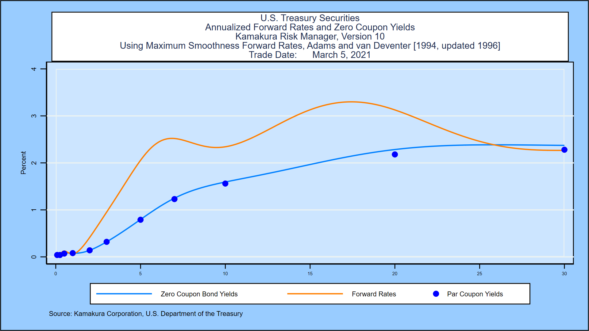
- The initial period 1 has no randomness, because the yield curve is observable as of March 5. In period 2, 91 days forward from March 5, shocks from the 10 factors will give us 500,000 different views of yields at the start of period 2.
- For period number J from 2 through 120, we do the following:
- Draw 500,000 normally distributed shocks for each of the 10 factors
- Calculate the interest rate volatilities that prevail at time step J in scenario K (since they will be dependent on the level of the prior period yield curve. Of course, at time step 2, there was only 1 prior yield curve, but from time step 3 onward, there are 500,000 prior yield curves)
- Multiply the volatilities times the 10 shocks and add those movements in forward rates to the forward rates of the prior period to get 500,000 new yield curves for time step J+1.
- If J is 120, stop. If J is less than 120, go to 4(a) and repeat.
Because HJM constraints on risk-neutral drifts in forward rates were strictly imposed, the Monte Carlo simulation for both models perfectly prices the initial U.S. Treasury yield curve for every possible forward time horizon, not just the first time step forward.
The following table compares the standard deviations of simulated interest rates at various time horizons:

The rates displayed are the “empirical” or “real world” interest rates that a risk manager would use to simulate value-at-risk or net income. The risk neutral rates are used for valuation. As we show in our March 11, 2021 report on the 1962-2020 Heath Jarrow and Morton model for U.S. Treasuries, the empirical distribution of rates gradually deviates from the risk neutral distribution. Neither distribution is normally distributed because the interest rate volatilities are not constant, but, of the 2 distributions, the empirical distribution is the “least normal,” bunching up near zero with a long tail of the distribution as rates rise.
We summarize the results as follows. Let’s start with line 1, the simulation of 3-month zero-coupon Treasury yields 1 year forward. The base model is the 10-factor HJM model. Over 500,000 scenarios, the mean 3-month yield is 0.076%. For the comparison model, the mean is close at 0.083%. The standard deviation in the base model is 0.232%, compared to 0.090% in the 1-factor model. That seems small at first glance, but the false assumption that only 1 factor drives interest rates reduced the “perceived risk” as measured by the standard deviation by 61.2%. The absolute differences are larger and more important as the maturities increase and the simulation time horizon increases. For the 10-year zero-coupon bond yield 15 years forward, the average level simulated using the 10-factor model was 4.100%. For the 1-factor model, the average of all scenarios was 3.080%, 102 basis points different. The standard deviation of the 10-year zero-coupon bond yield 15 years forward was 2.136%. Using the 1-factor model, the standard deviation was 0.343%, an understatement of the “true” risk of 83.9%.
Another way of stating the difference in risk assessment for the 10-year yield 15 years forward is this expression: The true risk is 6.23 times larger than what the users of a state-of-the-art 1-factor model would have reported.
How and why does this understatement of risk come about? Put simply, it is because a decision to use a 1-factor model ignores 9 other risk factors that a principal components analysis reveals. We elaborate in the next section.
3. Understanding Why a 1-Factor Model So Seriously Understates Risk
Consider the case of a 2-factor model. Let the short rate and the long (30-year) quarterly forward rate represent the two risk factors. If they were 100% correlated (positively or negatively), the second factor would not be needed. We consider the case where the 2 factors are correlated and we discuss just 2 scenarios, not 500,000:
Short rate up, long rate down
When the short rate moves up and the long rate moves down, there is a yield curve twist that a single factor model can’t “see.” In modern HJM interest rate models, the future path of interest rates is determined by both the choice of volatility functions and the shape, particularly the slope, of the yield curve. This up/down twist lowers the upward trajectory of rates and shifts the distribution of forward rates downward relative to a one factor model.
Short rate down, long rate up
This down/up twist increases the upward trajectory of rates and shifts the distribution of forward rates higher relative to a one factor model.
The result of a large number of twists is a higher degree of future interest rate volatility than a 1-factor model can generate even though both models have the same first factor and the same volatilities for that factor. As this excerpt from the Kamakura U.S. Treasury model shows, interest rate twists occur on 83.65% of the business days but 1-factor models ignore those twists:

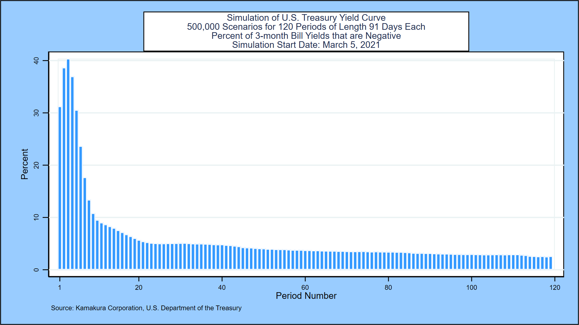
Another very important impact from the choice of a 1-factor model is that the perceived probability of negative rates becomes much smaller. The simulation implications of 1-factor models versus “all factor” models are much easier to see in graphical comparisons, to which we turn in the next section.
4. A Graphical Comparison of 1-factor and 10-factor Term Structure Models
At first glance, 1-factor models seem intuitively appealing, much like the often-heard quote “If you can’t explain the subject simply, you don’t understand the subject.” The correct expression is “If you can’t explain the subject simply, either you don’t understand the subject, or the subject is more complicated than most people assume.” By assuming a 1-factor model is true, all yield movements are either 100% or -100% correlated. If all interest rate volatilities are positive, that means all rate movements are 100% correlated and that all shifts of the full curve are in the same direction. In that model, all duration hedges work perfectly.
Here is a sample of 10 forward rate curves 5 years forward in the 1-factor model for March 5, 2021:
![]()
By contrast, 10 forward rate curves 5 years forward in the 10-factor model reflect the multiple factors that exist in reality and that lead to yield curve twists:
![]()
These two graphs alone make it clear how dramatically a 1-factor model can understate true risk.
We now display the probability distributions for 3-month zero-coupon yields and 10-year zero-coupon yields at various maturities. In all cases the distributions displayed are for the empirical or “real world” interest rates.
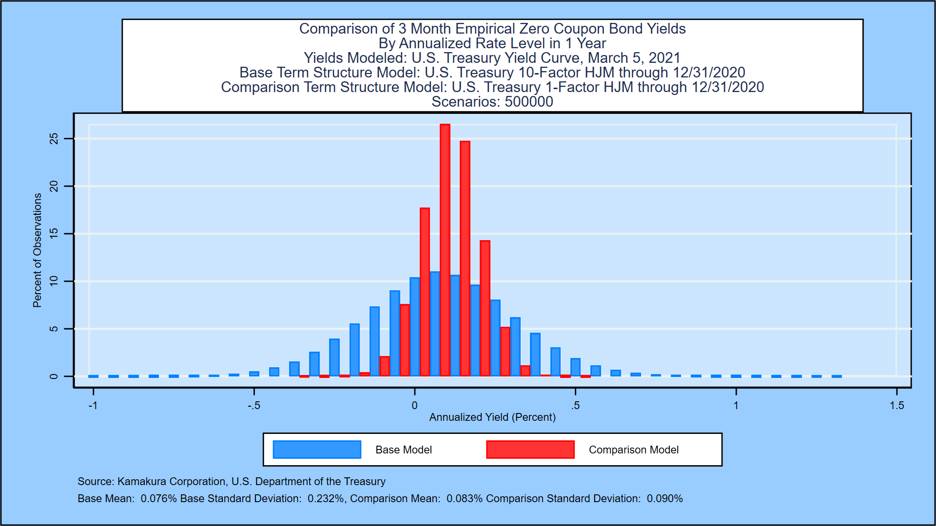


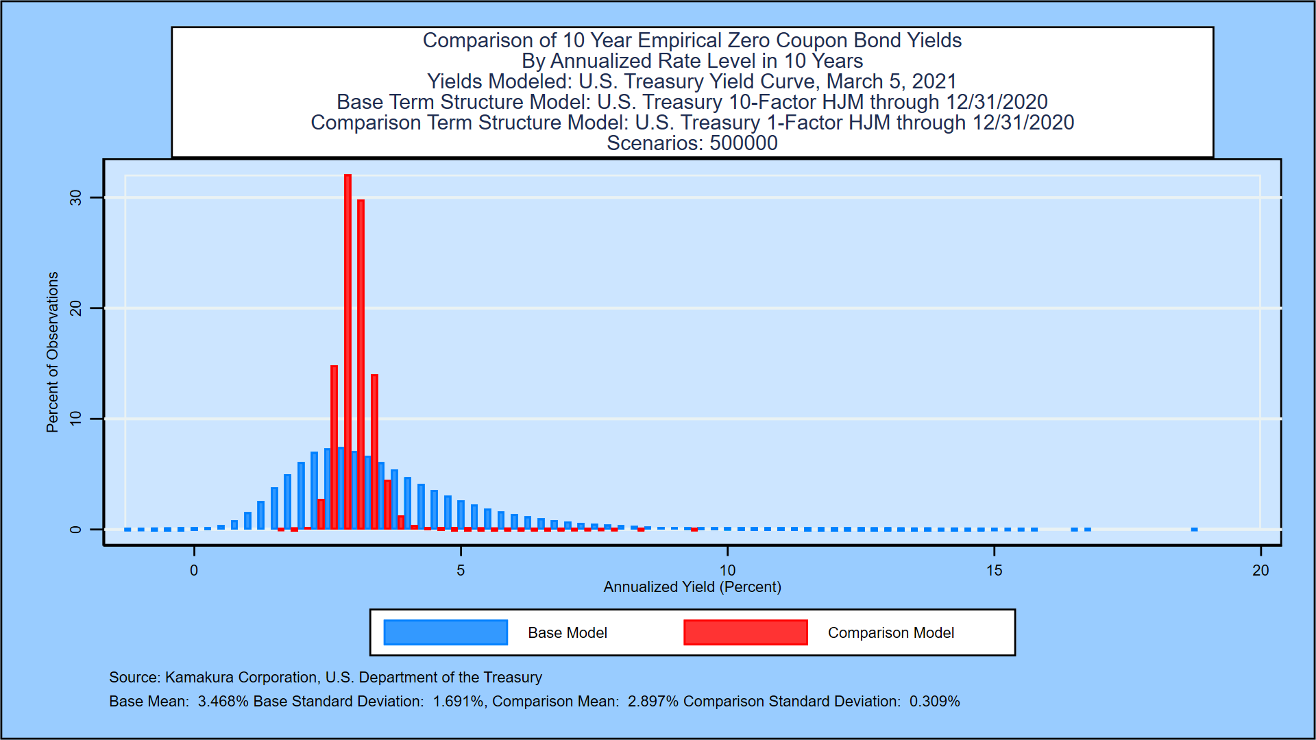

Finally, we compare the probability of negative 3-month empirical yields for the two models. As the probability graphs below show clearly, the 1-factor model dramatically understates the probability of negative rates over the simulation horizon.
1-factor Model Probability of Negative Yields at Each Time Step

10-factor Model Probability of Negative Yields at Each Time Step
5. Conclusions
A careful comparison of state-of-the-art Heath Jarrow and Morton 1-factor and 10-factor models of U.S. Treasury rate movements yields some significant conclusions:
- 1-factor model simulations understate the true level of future interest rate volatility
- 1-factor model simulations understate the future levels of interest rates except at very short forward time horizons
- 1-factor model simulations understate the probability of negative rates at nearly all time steps
We created an apples-to-apples comparison of two models benchmarked in the same manner on the same interest rate history using the same HJM-consistent assumptions on a third-party statistical package in wide use. The only difference in the models is the number of factors analyzed. Since all modern no-arbitrage rate models, with or without interest rate jumps, are special cases of HJM, these conclusions should be important to regulators, to members of the Boards of Directors, to senior management, and to shareholders. For risk managers, the implications are that multiple factor models are critical to an accurate measurement of interest rate risk.
REFERENCES
Adams, Kenneth J. and Donald R. van Deventer, “Fitting Yield Curves and Forward Rate Curves with Maximum Smoothness,” Journal of Fixed Income, 1994, pp. 52-61.
Adrian, Tobias, Richard K. Crump and Emanuel Moench, “Pricing the Term Structure with Linear Regressions,” Federal Reserve Bank of New York, Staff Report 340, August 2008, revised August 2013.
Jarrow, Robert A. and Kaushik Amin, “Pricing Foreign Currency Options Under Stochastic Interest Rates,” Journal of International Money and Finance, 10(3), September 1991.
Jarrow, Robert A. and Kaushik Amin, “Pricing American Options on Risky Assets in a Stochastic Interest Rate Economy,” Mathematical Finance, 2 (4), October 1992.
Campbell, John Y, Andrew W. Lo, and A. Craig McKinley, The Econometrics of Financial Markets, Princeton University Press, 1997.
Gelman, Andrew and John B. Carlin, Hal S. Stern, David B. Dunson, Aki Vehtari, and Donald B. Rubin, Bayesian Data Analysis, third edition, CRC Press, 2013.
Hansen, Bruce E. Econometrics, University of Wisconsin, January 15, 2015.
Hastie, Trevor, Robert Tibshirani and Jerome Friedman, Elements of Statistical Learning: Data Mining, Inference and Prediction, Springer, second edition, tenth printing, 2013.
Heath, David, Robert A. Jarrow and Andrew Morton, “Bond Pricing and the Term Structure of Interest Rates: A Discrete Time Approach,” Journal of Financial and Quantitative Analysis, 1990, pp. 419-440.
Heath, David, Robert A. Jarrow and Andrew Morton, “Contingent Claims Valuation with a Random Evolution of Interest Rates,” The Review of Futures Markets, 9 (1), 1990, pp. 54 -76.
Heath, David, Robert A. Jarrow and Andrew Morton,” Bond Pricing and the Term Structure of Interest Rates: A New Methodology for Contingent Claim Valuation,” Econometrica, 60(1),1992, pp. 77-105.
Heath, David, Robert A. Jarrow and Andrew Morton, “Easier Done than Said”, RISK Magazine, October 1992.
Ho, Thomas S. Y. and Sang-Bin Lee, “Term structure movements and pricing interest rate contingent claims,” Journal of Finance 41, December, 1986, pp. 1011-1029.
Jarrow, Robert A. Modeling Fixed Income Securities and Interest Rate Options, second edition, Stanford University Press, Stanford, 2002 and third edition, Chapman and Hall/CRC, 2019.
Jarrow, Robert A. and Stuart Turnbull, Derivative Securities, second edition, South-Western College Publishing, Cincinnati, 2000.
Jarrow, Robert A. and Yildiray Yildirim, “Pricing Treasury Inflation Protected Securities and Related Derivatives Using an HJM Model,” Journal of Financial and Quantitative Analysis 38 (2), June 2003.
Jarrow, Robert A. and Donald R. van Deventer, “Monte Carlo Simulation in a Multi-Factor Heath, Jarrow and Morton Term Structure Model,” Kamakura Corporation, Technical Guide, Version 4.0, June 16, 2015.
Jarrow, Robert A. and Donald R. van Deventer, “Parameter Estimation for Heath, Jarrow and Morton Term Structure Models,” Kamakura Corporation, Technical Guide, Version 4.0, May 5, 2017.
Kim, Don H. and Jonathan H. Wright, “An Arbitrage-Free Three Factor Term Structure Model and the Recent Behavior of Long-Term Yields and Distant-Horizon Forward Rates,” Finance and Economics Discussion Series, Federal Reserve Board, 2005-33.
Macaulay, Frederick R., Some Theoretical Problems Suggested by Movements of Interest Rates, Bond Yields, and Stock Prices in the United States since 1856, New York, Columbia University Press, 1938.
van Deventer, Donald R. “Essential Model Validation for Interest Rate Risk and Asset and Liability Management,” an HJM model for the U.S. Treasury curve, Kamakura Corporation working paper, www.kamakuraco.com, February 11, 2015.
van Deventer, Donald R. “Model Validation for Asset and Liability Management: A Worked Example” using Canadian Government Securities, Kamakura Corporation working paper, www.kamakuraco.com, July 20, 2016.
van Deventer, Donald R. “Interest Rate Risk: Lessons from 2 Decades of Low Interest Rates in Japan,” Kamakura Corporation working paper, www.kamakuraco.com, August 11, 2016.
van Deventer, Donald R. “A Multi-Factor Heath Jarrow and Morton Model of the United Kingdom Government Bond Yield Curve,” Kamakura Corporation working paper, www.kamakuraco.com, August 17, 2015.
van Deventer, Donald R. “A Multi-Factor Heath Jarrow and Morton Model of the German Bund Yield Curve,” Kamakura Corporation working paper, www.kamakuraco.com, August 21, 2015.
van Deventer, Donald R. “A Multi-Factor Heath Jarrow and Morton Model of the Australia Commonwealth Government Securities Yield Curve,” Kamakura Corporation working paper, www.kamakuraco.com, August 27, 2015.
van Deventer, Donald R. “A Multi-Factor Heath Jarrow and Morton Model of the Swedish Government Bond Yield Curve,” Kamakura Corporation working paper, www.kamakuraco.com, September 3, 2015.
van Deventer, Donald R. “Spanish Government Bond Yields: A Multi-Factor Heath Jarrow and Morton Model,” Kamakura Corporation working paper, www.kamakuraco.com, September 10, 2015.
van Deventer, Donald R. “Singapore Government Securities Yields: A Multi-Factor Heath Jarrow and Morton Model,” Kamakura Corporation working paper, www.kamakuraco.com, September 22, 2015.
van Deventer, Donald R. “The Regime Change Term Structure Model: A Simple Model Validation Approach,” Kamakura Corporation working paper, www.kamakuraco.com, January 26, 2016.
van Deventer, Donald R. “An 8 Factor Heath, Jarrow and Morton Model for the Japanese Government Bond Yield Curve, 1974 to 2016: The Impact of Negative Rates and Smoothing Issues,” Kamakura Corporation working paper, ww.kamakuraco.com, June 21, 2017.
van Deventer, Donald R. “A 10 Factor Heath, Jarrow and Morton Stochastic Volatility Model for the U.S. Treasury Yield Curve, Using Daily Data from January 1, 1962 through December 31, 2020,” Kamakura Corporation working paper, www.kamakuraco.com, March 11, 2021.
van Deventer, Donald R., Kenji Imai and Mark Mesler, Advanced Financial Risk Management, second edition, John Wiley & Sons, Singapore, 2013.
Vasicek, Oldrich A, “An Equilibrium Characterization of the Term Structure,” Journal of Financial Economics, 1977, pp. 177-188.
Woolridge, Jeffrey M. Econometric Analysis of Cross Section and Panel Data, The MIT Press, 2002.
Footnotes
[1] Kamakura Corporation, dvandeventer@kamakuraco.com. The author wishes to thank Professor Robert A. Jarrow for his patience and insights on HJM from 1995 onward. The author is proud to have been a student of Professor Jarrow for longer than any other of his students. The author also wishes to thank Kamakura colleagues Martin Zorn, Daniel Dickler, Theodore Spradlin, and Dr. Xiaoming Wang for assistance in the modeling effort.
[2] Exceptions are interest rate derivatives desks and bond trading desks. Our comment refers to enterprise-wide total balance sheet risk management.
[3] In the interest of full disclosure, Kamakura Corporation’s enterprise risk management system Kamakura Risk Manager has featured multi-factor interest rate risk models for more than 20 years.
[4] Government yield curves are modeled for Australia, Canada, France, Germany, Italy, Japan, Russia, Singapore, Spain, Sweden, Thailand, the United Kingdom, and the United States.
[5] Since the simulation will be done for 91-day time steps, and since the initial “spot” 91-day U.S. Treasury yield is observable at the current time, the “short rate” is the 91-day forward rate that spans a 91-day period from day 91 to day 182. The shock to this factor is its change from the initial forward rate to its level 91 days later, when the forward rate becomes the 91-day spot rate.
[6] If we had only 3 factors, the order of maturities used for the 3 factors would typically be (1) the shortest, (2) the longest, and (3) the middle. We follow that pattern.


